NOM
Mgraph
Mgraph [options] [command file]
DESCRIPTION
Mgraph is an ``easy to use'' graphic software
allowing a fast visualization of scientific data presented in
the form of ASCII files for the traditional curves, and in the
form of binary files for data surfaces.
The interface was
developed under Motif and can be used either interactively [page pageref],
or using with command files [page pageref],
or included in C or FORTRAN programs[page pageref].
The output files are in PostScript.
Images in Tiff or Gif format can also be generated.
Mgraph [options] starts of the interactive interface. Mgraph [options] file.com starts of the graphic interpreter without visualization.
OPTIONS
| Mgraph*FontList: "-Adobe-Courier-Bold-r-Normal-*-12-*-*-....." |
**********************************************************
**********************************************************
*
When installing Mgraph on your computer, the Mgraph.ad file is
placed in the system directory:
| /usr/lib/X11/app-defaults |
| xrdb -merge Mgraph.ad |
* The option -zoom can be integrated into Mgraph.ad;
For that purpose, modifies the line:
| Mgraph_bin*zoom: 100 |
| Mgraph*FontList: ``-Adobe-Courier-Bold-r-Normal-*-12-*-*-*-*-*-*-*'' |
In the panels, use the left mouse button to select the options, to
activate the push buttons or to point to a position on the request of
the software.
Any character string in an editor can be selected using
the same button and then pasted into another editor using the central
button.
In the graphic window:
Simple read
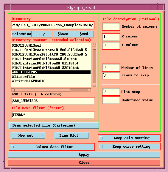
File selection
The input file is an ASCII file (or binary, or TIFF/GIF in Contour mode)
containing numbers in columns separated
by spaces, commas or tabulations.
The read function filters the data,
automatically skips the lines containing strings, and determines the
number of lines and columns to be drawn.
The working directory is shown in the editor at the top of the window. You can directly type a new directory in the editor (and carriage return) or click on the desired directory in the Unix file structure displayed.
ex:
| Type: | the head of the list will be: | |
| *data | all the files ending with ``data''. | |
| data* | all the files beginning by ``data''. | |
| *data* | all the files having ``data'' in their name. |
You have the possibility to select multiple files using the combination
of the mouse click and the SHIFT or CTRL key; in this case, the curves are added in the
graphic window.
The option ``Keep curve setting'' draws curves with the same type than the previous plot
(the color, line style and mark style).
The option ``Keep axis setting'' draws curves with the same limits of axes than the previous plot.
In order to preserve these limits for later sessions, it is enough to
activate the option ``Files->Save defaults''.
Description of the file
If the ``File description'' editors are not filled, the first column is
taken as X coordinate and all subsequent columns as various sets of Y
coordinates.
If the file contains only one column, data are drawing on the Y-axis and their line numbers
on the X-axis.
If the ``X column'' editor is set to zero, the line numbers will be on the X-axis.
By filling the editors you are able to:
Various options and plot modes are proposed.
Selection of the type of curve: Menu ``Line plot''
| Line plot | The adjacent points are joined by a line without any symbol. |
| Scatter plot | The points are represented by symbols without any connecting line. |
| Error Bars X | The file is read like a sequence of (X,Y,Delta), where Delta is the error on X. A horizontal bar of length 2*Delta centered in X,Y will be drawn. |
| Error Bars Y | Same curve with vertical error bars. |
| Step plot | the file is drawn as steps (i.e. Pseudo histogram). For
each point a horizontal line is drawn at the corresponding
Y-value, from the median of the X-values of that point and
the previous one to the median of the X-values of that point
and the next one:
X = [(Xn+Xn-1)/2] to X = [(Xn+Xn+1)/2]. |
Type of graph
Selection of the window plotting mode: menu ``New set''
| New Set | New plot. |
| Add mode | Keeps the plot setting and adds the new curves. |
| Replace mode | Keeps the plot setting and replaces the curves by new ones. |
| Merge mode | Keeps the plot setting and adds to the existing curves the new data points. |
Data filter
Column data filter
A new menu (Mgraph_column_data_read_filter) appears which allows you to enter
the filter command as:
| value < column number < value |
If many filters point on the same column, an exclusive OR is used, between several
columns a AND is performed.
Before starting the main read, click on ``Analyze user filter editor''
to valid the filter.
Selection of the processing
menu ``Draw selected file''
| Draw selected file (Cartesian) | Plots simple functions y=f(x). |
| Draw selected file (Polar) | Plots simple functions in polar coordinates. |
| Compute histogram of selected file | Plots the histogram of the various columns of the file. (See page pageref) |
| Statistics of selected file | Calculates and displays statistics (Average, standard deviation and so on) on the various columns of the file. |
| Digitalization | Digitalization of curves starting from scanner images or images visualized on the screen by any other software. (See page pageref). |
| File preview | The file is edited in a window ``Mgraph_preview''. |
| Draw surface contours | This menu allows reading of surfaces in various formats (ASCII, TIFF, GIF or binary) and carries out the interpolations making it possible to calculate isovalue lines and projections. (See page pageref) |
Several formats of file surface exist:
Signed This option is used only for the integer words. Cut values allows you to filter values. Stretch Z values allows you to change Z values.
|
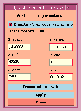
| Build a surface from XY Data | From an ASCII file containing X,Y data, Mgraph computes a surface from boxes of variable size containing percentage of points. |
| Import a new lut | Loads the user color base with a new look-up table. These LUTs are used only by the contour routines. Two formats are decoded: |
|
| Draw arrows | From an ASCII file, vectors are definite from their origins (X and Y), their length (Rho), their orientation (Theta) with possibility of changing the arrow size (Length and Arrow factor). |
If you have selected a file, activate ``Apply'' to display the result.
Specific read
According to the selected options, the following windows could be
displayed:
| Compute histogram of selected file |
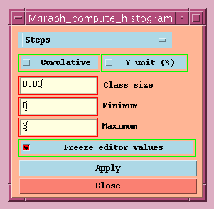
You are able to define the type of curve, the limits of the histogram, the width of the classes, the units in Y. Warning: if you modify the editors don't forget the option ``Freeze editor values'' before doing ``Apply'' to avoid the automatic calculation.
| Digitalization |
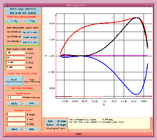
If the selected file is a TIFF or GIF file, the function ``Apply'' will read and
display the image in the digitalization window. If not, you have the
possibility, by using the function ``Grab image from display'', to pick and
slide an image on your screen by using the mouse (image presented by other
software such as ghostscript, for example). The window under the image
displays messages and directives.
N.B. The image is shown in black and white. You can choose the color
visualization with the ``Switch image (BW/Color)'' button
The digitalization is done in several steps:
Warning! The smooth and sampling affect only the last digitalized curve.
| File preview |
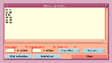
Visualizes the contents of the file in a window and then allows you to
select with the mouse one set of lines to be plotted with the selected
options.
| Draw surface contour |
Show the surface and then allows you to select many parameters. (See lower ``FILES->SURFACE & CONTOUR'' §1.1.4).
| Build a surface from XY Data |
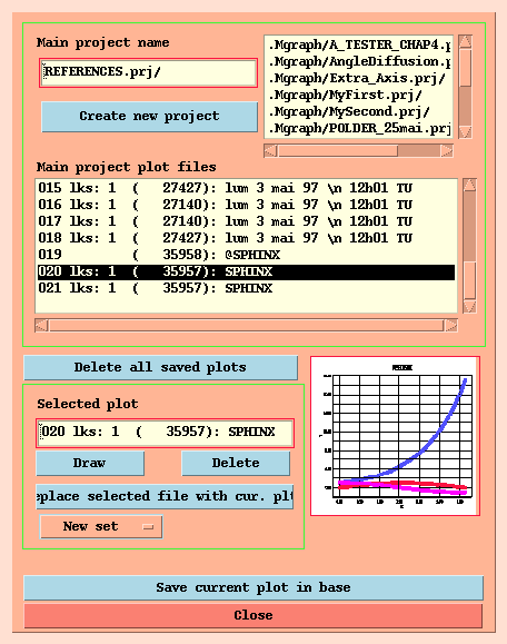
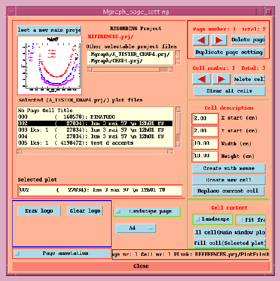
The user has the option of managing various directories (``Main project name'')
containing the graphic files and the page setting files built
during a session.
The list of the directories appears in the upper right corner of the
window. Selecting a directory name in this window becoming Mgraph
working directory (Main project).
Its contents are displayed in the window ``Main project plot files''.
(If a graph is used in a page setting, it appears
with a link [lks: 1]. See also the menu ``Settings->Page setting'' §1.2.6).
To create a new project, it is necessary to type its name in the editor
and to activate ``create new project''.
Options:
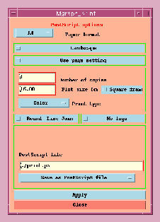
With this menu, you can send your work to a printer or save it as
PostScript (or Encapsulated PS) file, using the main graphic window or using a page setting
containing several plots.
Options:
| LOGO_FILE /usr/my_directory/mylogo.eps |
Note: You can introduce your own signature in the
lower right corner of the page by modifying the line of
the .Mgraph/MgraphDefaults file:
| type: | for: | |
| SIGNATURE | "L.O.A. Computer Team" | Date + signature |
| SIGNATURE | " " (Spaces) | Date |
| SIGNATURE | "" (Empty) | nothing |
| lp -dPRINTER |
When you have defined your printers, activate the option ``Save defaults'' to back them up.
This menu allows surface interpolations to compute isovalue lines and projections. It can be activated only if the user has already stored a surface using the menus ``Files->Read files->Draw surface contours'' or ``Files->Save & restore->Draw''.
The menus ``Mgraph_surface_view'' and ``Mgraph_surface_geometry'' appear.
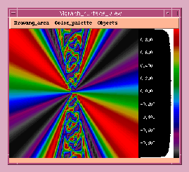
This window does the surface visualization. On the right side an
histogram of the values is drawn. Various options are available:
| Drawing_area->Zoom | Enlarge a part of the image. |
| Drawing_area->Show values | Show the Z values of the surface. |
| Drawing_area->Rescale | Show the original image. |
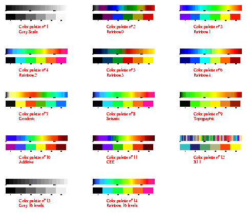
| Color_palette-> | Internal color look up tables. |
| Color_palette->User Lut Base | User's data files containing color scales (See the menu ``Read files->Import a new lut''). |
| Color_palette->Grey scale etc... | Basic color scales of Mgraph (description §1.2.8) |
| Objects->Clear all | Clear all options. |
| Objects->Draw triangles | Show the triangles used in the interpolations. |
| Objects->Draw region | Show the computed areas separating the real points from the undefined points introduced by the options ``Undefined value'' or ``X Y Z irregular grid'' of the reading menu. |
| Objects->Draw points | Show the measurement points. |
| Objects->Draw all | Show all the options. |
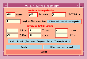
allows the user to modify:
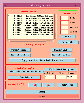
This menu allows the user to draw the isovalue lines. The software predetermines some values of contours to be plotted. Click on ``Apply'' to run calculation and to plot the curves whose presentation can be modified in the menu ``Settings->Plot settings''.
To enter its own list of values it is necessary to:
The styles of the curves are determined by the various menus of ``Isoline plot style''. If the option ``Current color'' is chosen, colors are predetermined by the software.
Modification of the plot options of one or several isovalue lines:
Select the value with the mouse,
then select in the different items the drawing options (color,
type of line, symbol, labels ).
Activate ``Apply new style'' the parameters are modified in
the editor. The new presentation will appear on the graph by
activating the main ``Apply'' located at the bottom of the menu.
If the isovalue lines are drawn with the option ``Label'' you can change,
by using the menus of the ``Label plot style'', the
presentations (foreground or background color, distance between
2 labels).
The modifications appear by activating the main ``Apply'' of the menu.
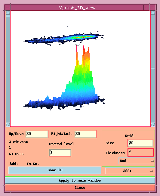
This menu allows you to draw a 3D view of the computed surface displayed
on the main window.
The window Mgraph_3D_view can project the surface into
the graphic window with the ``Apply to main window'' button.
for this addings, click on ``Apply to main window''.
You may modify the 3D level and its position in the window with two scrollbars (right and left). Click on ``Show 3D'' to show the result.
This menu allows you to come back to the 2D surface. You must clear the 3D view to read a new image.
Creates a command file as near as possible to the required graphical presentation for a simple curve or a page setting. It will allow the use of Mgraph in the non-interactive mode (see §1.6).
Creates an Encapsulated PostScript file for inclusion in Word or TeX documents.
Creates an ASCII file containing the coordinates of the different visualized curves. You can directly read again this file with Mgraph (menu Files->ReadFiles) to redraw the plots.
The word ``Break'' breaks the continuity of a curve
(Countour plotting for example).
The word ``NewCurve'' adds a new curve.
A line ``CURVE NUMBER:... separates the different curves, it
is automatically skipped by the software with the second
reading.
Options:
``Create new file'' performs the extraction.
Creates a file in TIFF or GIF format representing the graphic window. This image can be read by various types of visualization software or image format converters. drawing.tif is the default name.
A file `` ~ /.Mgraph/MgraphDefaults'' contains your options:
| LOGO_FILE | Myfile.eps | |
| LOGO_POSX | 1 | |
| LOGO_POSY | 2.7 | |
| LOGO_SCAX | 0.14 | |
| LOGO_SCAY | 0.14 |
| SetSignature | "My signature" |
==========================================================
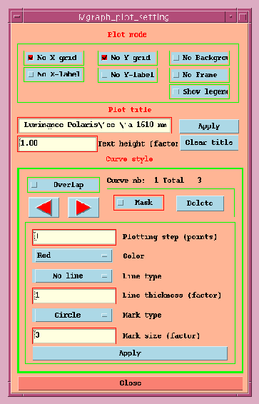
This menu allows you to modify the style of each visualized curve and to modify the plot setting.
These options allow you, with immediate effect on visualization, to include (or remove) grids, labels, legend, 2 axes or 4 and the surface(``No Background'').
Modifies the title; to activate this menu, you can also click on title zone.
By activating the option ``Overlap'', the curves are presented
together, which allows the modification of a parameter for all
curves in one action.
parameter types:
If the option ``Overlap'' is unselected, the curves will be shown one by one. In this mode you can mask or remove a curve.
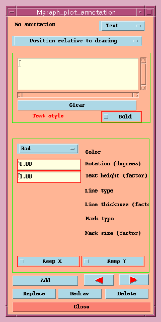
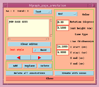
This menu allows you to annotate the graphic window.
The graphic window can be empty of surface or plot drawing. See its utility in §1.2.9.
Various additions are possible:
text, symbol, line, box, arrow and extra axis plots.
For each annotation, you can choose:
For each one, you have to select the color and the type.
In the case of
multiple annotations, you have the possibility to freeze the X or Y
value. Activate Add and use the mouse to select position in the
graphic window .
Replace allows you to reposition the annotation;
Redraw allows you to redraw the annotation in the same place;
Delete removes the annotation;
(See also in F.A.Q §3.4 the characters codification).
The annotation ``Extra axis'' allows you to draw an additional axis, or to
replace one of the existing axes by a new one completely independent of
the limits of the curve. In the axis editors the value of the ``mini''
can be higher than the ``maxi''; for an axis plotted using the mouse, the
``mini'' will be at the first selected point (see F.A.Q [3.4]).
Click on the button Free labels, allows you to label axis with a list:
the axis value following by a text between quotes or an independant value
written with the given format.
Simply click on the annotations to make this menu appear.
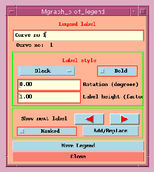
When this menu is called, the legend is visualized in the upper left corner of the graphics window. Each curve is represented (except the masked curves - see ``Plot Setting'' [1.2.1]). You can annotate, rotate the text, or mask each legend. The button ``move legend'' allows you to move and resize the legend.
This menu allows you to add a color scale into the graphic window.
The graphic window can be empty. See its utility in §1.2.9.
Two styles of color scale are proposed:
This option allows you to quickly draw a linear color scale.
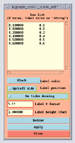
This menu allows you to mark colored boxes with a label. Like for the linear color scale, you can choose between formatted value and text. The option ``Redraw'' redraw the scale with chosen options. The option ``Apply'' moves and draws the scale.
This option clears all color scales.
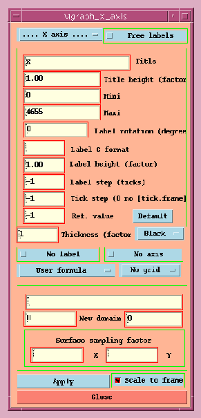
This menu can also be called by clicking with the mouse on the center of the axis annotations, or in the lower left corner of the graphic window. For each axis, the editors allow you to set:
| precision: | number of decimals for the formats f, e and E |
| number of digits for the formats g and G (6 per default) | |
| conversion: | g universal notation (i.e. d, f, or e) |
| G universal notation (i.e. D, F, or E) | |
| f decimal notation (i.e. ' [-]dddd.ddd') | |
| e exponential notation (i.e. ' [-]d.ddde+dd') | |
| E exponential notation (i.e. ' [-]d.dddE+dd') |
example:
| 12.65978 | %g | � 12.6598 |
| %f | � 12.659780 | |
| %.3f | � 12.660 | |
| %.2e | � 1.27e+01 | |
| %.0f | � 13 | |
| %+.1f | � +12.7 | |
| 12.00 | %g | � 12 |
It's possible to undraw the labels (``No X-label'' item), to choose tics or
grids (standard or half-tone) on the axes (``Std grid'').
You may cut out an axe (``No axis'').
Several types of axis are proposed: linear, logarithmic , calibrated in
time or decimal degrees but also transformed by a user equation.
In
this case, the original data are not transformed; only its graphic
presentation is modified. Type a formula in the formula editor. This
formula will be backed up and a list of equations will be created
(listed in the panel Mgraph_formula_list).
You may adjust the function domain of the projection to avoid, for
example, dividing by zero.
For more details, see §1.3.2 menu Math->Formula.
For each axis, you may define the tickness and color.
This menu enables you to create interactively a page presentation with
graphics.
The presentations are saved in the same user database (see
``Files->Save&Restore'' §1.1.2).
Each annotation may be positioned using the mouse ``Fill editors
with mouse'' or directly by filling the editors.
The options ``Add'', ``Replace'' and ``Delete'' visualize the annotations on the page.
To print this page, activate menu ``Files->Print plot'' with the
function ``Use page setting'' activated.
This page can also be exported in a command file for an automatic production.
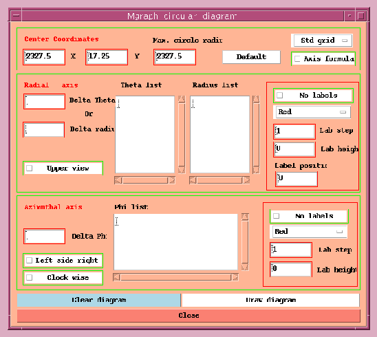
This menu allows you to replace axis drawing by a diagram composed of
circles and radius. The options define:
| Delta Theta | circle step in degree. |
| Delta radius | circle step in main radius unit. |
| Theta list | free list in degrees. |
| Radius list | free list in main radius unit. |
| Delta phi | radius step in degree. |
| Phi list | free list in degree. |
| Upper view | upper view of the sphere. |
| Left side right | radius origin is at left or right. |
| Clock wize | radius drawing in clock wise. |
| Axis formula | uses of projection fixed in axis definition. |
and various parameters of labels drawing on circles and radius (color, size and position).
The graphic window can be empty of curves or surface. See its utility in §1.2.9.
In this case, click on ``Default'' or ``Draw Diagram'' button and
the editors (X,Y, Radius) will be filled with the value 0.5.
User LUT base:
From the user's LUT base, this menu loads a new LUT.
Click on the filename, its contents will be shown at the right side.
The lines in the file beginning with the character # will not be read.
Two formats are decoded:
|
|
Mgraph gives the possibility to create a window WITHOUT CURVE NOR SURFACE,
with annotations, color scale or circular diagram.
This window is used in a ``Page setting'' (§1.2.6),
for example, to show a common color scale to many images in differents cells.
This window can be saved as standard windows. It will be registred as ``@Annotation window''.
Its scaling is defined by the software as 0. to 1. for X and Y.
==========================================================
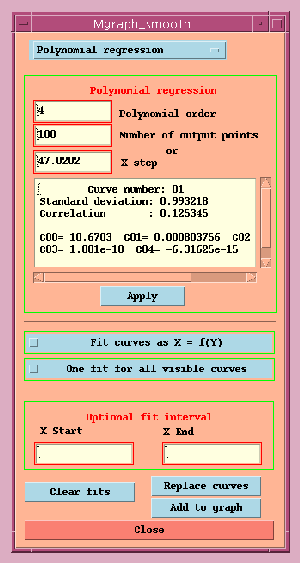
The following options are common to all mathematic sub-menus:
The regression is done as y = f(x) by default but you can choose x = f(y).
You can also select to fit all the curves as an independent sets of
data (the default) or as one set of data.
You can choose the domain of fit: the default is the data
visible in the graphic window.
You can select the sampling of your resulting curves. (ex: the
fit domain can be a little extended to do an extrapolation of
the data).
The resulting curves can be added to the original curves or
replace them.
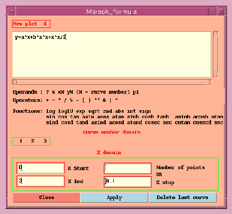
This menu allows to process operations on the curves.
The operands are: ``xN'' and ``yN'' (where N is the curve number),
'pi' and 'x' to use the X domain editors.
The operators are: ' = ' , '+' , '-' , '*' , '/', '%', '**',
'(', ')', '&' (and), '|' (or), '^' (xor).
The functions are the standard mathematical functions (see
§2.3). 'rnd()' generates a random number between 0 and 1.
You can compute new curves by filling the editors ``X domain'':
example: y = sin(x) with Xstart = 0, Xend = 3.14 and Number of points = 100
then ``Apply'' will create the plot.
You are able , in the same way, to resample an existing curve : Type in
the equation editor: x1 = x1 and fill the ``X domain'' editor with the
sampling X values.
All the equations are saved and listed in the widget ``Mgraph Formula list'. You have to use this list to cut and paste lines for the ``Formula editor''.
The Fast Fourier Transform allows you to filter a curve, finding the
most significant frequency components. Each component is displayed with
the coefficient of correlation calculated between the data and the
inverse FFT with this frequency suppressed.
This menu also enables you
to remove, multiple frequencies (``Reduce spectrum'') or frequency by
frequency (``Delete a component'').
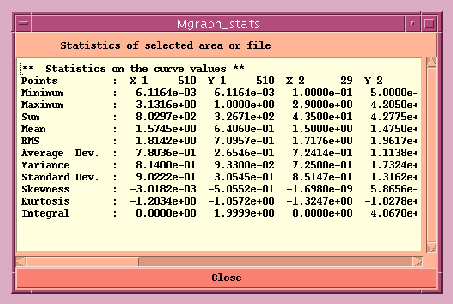
This menu computes average, standard deviation and so on, on the visible curves of the graphic main window.
From an ASCII file containing X,Y data, Mgraph computes a surface from boxes of variable size containing percentage of points.
==========================================================
This menu allows you to initialize the main graphic window. All the curves and the plot setting will be cleared.
This menu allows you to create a new independent graphic window. You can open up to 10 windows simultaneously. The small red square in the upper left corner of the window indicates which one is active. Warning! Mgraph ``Quit'' function closes all the opened windows and stops the run.
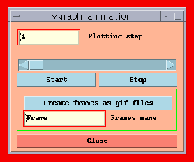
This menu allows to animate the curves plotted in the main graphic window to visualize, for example, time effects.
==========================================================
Allows the user to delimit a set of points within a range of
values by clicking with the right mouse button.
This function is also called by clicking on the small red square
in the upper left corner of the graphic window.
(The green square is used to rescale the graphic window after a
``zoom'')
Shows the coordinates of the points selected by the right mouse button. To quit the function click on the left mouse button.
This option rescales the plotting area to include all the
plotted data points after a ``zoom'' or after an equation
transformation.
This function is also called by clicking on the small green
square in the upper left corner of the graphic window.
Allows you to erase plotted data points. Caution! The selection box must be sufficiently large. If you wish to remove only one point, it will perhaps be necessary to increase the zone (zoom) before selecting ``Clear area''.
Allows you to store in a file the points selected by the
mouse button. The file name default is ``values.data''. This
file name is incremented with each activation of the function:
values01.data, values02.data , and so on...
The file is in ASCII format: 2 columns (X-coordinate,
Y-coordinate).
``Apply'' activates a window displaying the coordinates.
The selected point is recorded when the left mouse button is
pressed.
To quit the function, click on the right mouse button.
==========================================================
French or English Help on line
**********************************************************
**********************************************************
In this mode, graphics are generated in an automatic way without
visualization.
An option Mgraph -show fich1.com can be used;
in this case, after the
last plot, the Motif version of the software will start and the last
curve will appear in the main graphic window.
A command file can be parameterized in a very simple way using a system
of aliases (Free Word preceded by the character @). This allows to
replace whole or part of a command by a line introduced into the data
file.
Ex: in the command file aa.com we have:
Switches the dimensions and coordinates to inch units (centimeter by default).
where Filename is the name of the EPS file containing the logo.
Prints "text" as a page signature.
Specifies the graphic window geometry.
STYLE=LinePlot|ScatterPlot|ErrorBarsX|ErrorBarsY|Stepplot
[ NCOLUMNS=-1 XCOLUMN=-1 YCOLUMN=-1 NLINES=-1 ]
[ ERRORCOLUMN=-1 LINESTOSKIP=-1 UNDEFVALUE=-1 ]
[ NCOLUMNS=-1 XCOLUMN=-1 YCOLUMN=-1 NLINES=-1 ]
[ LINESTOSKIP=-1 UNDEFVALUE=-1 ]
MODE=Normal|Cumulative YUNIT=Density|PerCent
[ NCOLUMNS=-1 YCOLUMN=-1 NLINES=-1 ]
[ LINESTOSKIP=-1 UNDEFVALUE=-1 ]
[ XMIN=-1 XMAX=-1 CLASSSIZE=-1 ]
DATATYPE=8bit | 8bitsigned | 16bit | 16bitsigned | Integer | Float
STYLE=LinePlot|ScatterPlot|ErrorBarsX|ErrorBarsY|Stepplot
NCOLUMNS=-1 XCOLUMN=-1 COLUMN=-1 NLINES=-1
[ ERRORCOLUMN=-1 LINESTOSKIP=-1 UNDEFVALUE=-1 ]
[ NCOLUMNS=-1 NLINES=-1
LINESTOSKIP=-1 UNDEFVALUE=-1]
[ DISTANCEFACTOR=-1 ZMIN=-1 ZMAX=-1 ]
DATATYPE=8bit | 8bitsigned | 16bit | 16bitsigned | Integer | Float
NCOLUMNS=-1 NLINES=-1
[ UNDEFVALUE=-1 DISTANCEFACTOR=-1]
[ ZMIN=-1 ZMAX=-1 ]
NCOLUMNS=-1 NLINES=-1 XCOLUMN=-1 YCOLUMN=-1
XMIN=-1 XMAX=-1 XSTEP= -1
YMIN=-1 YMAX=-1 YSTEP=-1
[ LINESTOSKIP=-1 UNDEFVALUE= -1 ]
NCOLUMNS=-1 XCOLUMN=-1 YCOLUMN=-1
NLINES=-1 LINESTOSKIP=-1
RHOCOLUMN=-1 THETACOLUMN=-1
LENGTHFACTOR=-1 ARROWFACTOR=-1
example:
XGRID=Yes|Light|No YGRID=Yes|Light|No
[ MIN=-1 MAX=-1 DELTA=-1 LABEL=Yes|No ]
[ FORMULA="my_formula" NEWXMIN=-1 NEWXMAX=-1 ]
LABELHEIGHT=1 CFORMAT="format" ANGLE=0.
LIST= value1 "texte1" ... valueN "texteN"
[ MIN=-1 MAX=-1 DELTA=-1 LABEL=Yes|No ]
[ FORMULA="my_formula" NEWXMIN=-1 NEWXMAX=-1 ]
LABELHEIGHT=1 CFORMAT="format" ANGLE=0.
LIST= value1 "texte1" ... valueN "texteN"
[ MIN=-1 MAX=-1 DELTA=-1 LABEL=Yes|No ]
[ FORMULA="my_formula" NEWXMIN=-1 NEWXMAX=-1 ]
LABELHEIGHT=1 CFORMAT="format" ANGLE=0.
LIST= value1 "texte1" ... valueN "texteN"
[ GRID=Light DEPEND=AxisFormula ]
LABEL=Yes|No LABELSTEP=-1 LABELHEIGHT=1
[ UPPERVIEW=Yes|No ] LABELPOSITION=-1 COLOR=Black
where LabelPosition= is position of radius labels in degrees.
LABEL=Yes|No LABELSTEP=-1 LABELHEIGHT=-1
COLOR=Black [ CLOCKWISE=Yes|No ORIGIN=LeftSideRight ]
[ MIN=-1 MAX=-1 ] WINDOWSIZE=-1 STEP=-1
[ MODE=Add|Replace|Merge VARIABLE=X|Y ]
[ MIN=-1 MAX=-1 ] WINDOWSIZE=-1 STEP=-1
[ MODE=Add|Replace|Merge VARIABLE=X|Y ]
[ MIN=-1 MAX=-1 NPOINTS=-1 STEP=-1]
[ MODE=Add|Replace|Merge VARIABLE=X|Y ]
[ MIN=-1 MAX=-1 NPOINTS=-1]
STEP=-1 ORDER=1
[ MODE=Add|Replace|Merge VARIABLE=X|Y ]
FIT_RESULT_AS_ANNOTATION=Yes|No
XSTART=0 YSTART=0
COLOR=Black STYLE=Plain|Bold HEIGHT=1
[ MIN=-1 MAX=-1 NPOINTS=-1 STEP=-1 ] ERROR=1.e-05
[ MODE=Add|Replace|Merge VARIABLE=X|Y
FORMULA=Ëquation" INIT=Ïnitial values"
FIT_RESULT_AS_ANNOTATION=Yes|No
XSTART=0 YSTART=0
COLOR=Black STYLE=Plain|Bold HEIGHT=1
WARNING!
BACKGROUND=transp|white
FOREGROUND=Undef|White|Black
CFORMAT="format" SIZE=1
LINESTYLE=Solid MARKSTYLE=Bigdot
DISTANCEFACTOR=-1 XYRATIO=-1 INTERPOLATION=Yes|No
STRETCH=0.93 SHIFT=0.09 GRIDSIZE=40.
COLOR=Black THICKNESS=1.
where Zmin,Zmax are the minimum and maximum values (Z) of the surface. This
interval will be divided into 256 color levels.
where FirstLevel and LastLevel are the interval values of the LUT ( 0 to 255) used for the
level division V1 V2.)
The following commands can be used in an ``Annotation Window''.
where LutNumber= is the internal color LUT type between 1 and 14 (description §1.2.8)
if filename exist, the ASCII file "File_name" is decoded.
2 types of LUT :
XSTART=-1 YSTART=-1 XEND=-1 YEND=-1 MIN=-1 MAX=-1
COLOR=Black POSITION=DownRight|UpLeft
NOTICK=Yes|No CFORMAT="format" SIZE=1
LIST= Z0 Label0... Zn Labeln
where XStart.... YEnd are the coordinates of the rectangle. They are given
in user units or expressed as a percentage of the size of the axes in
this case numbers are followed by the character %.
where Min Max (0->255) are the boundaries of the color LUT to be plotted.
(If you want to mask a part of the LUT).
where z0 label0.. are the z value following by label (value or text)
COLOR=Black STYLE=Plain|Bold
HEIGHT=1 ANGLE=0 TEXT="text to plot"
COLOR=Black STYLE=BigDot SIZE=1
COLOR=Black STYLE=BigDot THICKNESS=1
COLOR=Black STYLE=Solid THICKNESS=1
COLOR=Black STYLE=Solid THICKNESS=1
[ XSTART=0 YSTART= 0 XEND=0 YEND=0]
SCALE=Linear|Logarithm|Time|Degree|Formula
[ FORMULA="my_formula"]
MIN=0 MAX=0 DELTA=0
COLOR=Black THICKNESS=1
TITLE="Title of axis" TITLEHEIGHT=1
LABEL=Yes|No POSITION=UpRight|DownLeft LABELSTEP=-1
[ REFERENCE=-1 LABELHEIGHT= 1 CFORMAT="format" ANGLE=0]
[ LIST= value1 "texte1" ... valueN "texteN" ]
COLOR=Black STYLE=Plain|Bold
HEIGHT=1 ANGLE=0 TEXT="text toplot"
COLOR=Black STYLE=Solid THICKNESS=1
COLOR=Black STYLE=Solid THICKNESS=1
TYPE=Black&White|GrayScale|Color
[ ORIENTATION=Landscape|Portrait MODE=ScaleToFrame|Margin ]
[ SIZE= 15 COPIES=1 ORIENTATION=Landscape|Portrait ]
[ ORIENTATION=Landscape|Portrait ]
[ SIZE= 15 COPIES=1 ORIENTATION=Landscape|Portrait ]
This command transfers the result to a PostScript viewer:
Ex: SendToDisplay ghostscript
Exp, log10, log, sqrt, rnd()
sign, abs, int,
sin, cos, tan (in radian),sind, cosd, tand (in degrees)
asin, acos, atan, asind, acosd, atand,
sinh, cosh, tanh,
asinh, acosh, atanh,
cosec, sec, cotan, cosecd, secd, cotand
+, -, *, / , % (integer division),
** (power)
& (AND) , | (OR) , ^ (XOR), ~ (complement)
You are able to run this example by copying it in a file (a.com) and by
running the command Mgraph -show a.com.
2.1 GENERAL CONTROLS
N.B. Mgraph interactive mode creates the file from the simple
graphic window or from the complex page setting.
So, you have just to change a few parameters if necessary.
The command can be: Mgraph fich1.com or Mgraph fich1.com fich2.com and so on..
		Verbose
		SetAlias
		ReadFile      File="./data"
		PlotTitle     Title="@TITLE"  Height=1.20
		@STYLE
		etc.
In the file ``data'' we have:
		@TITLE  Data 12-10-97
		@STYLE LineStyle Curve=1 Style=MicroDash Color=Red Thickness=2
		0 	0
		100 	-1
		150 	1
		etc.
The command file finally executed will be
		Verbose
		SetAlias
		ReadFile      File="./data"
		PlotTitle     Title="Data 12-10-97"   Height=1.20
		LineStyle     Curve=1  Style=MicroDash  Color=Red   Thickness=2
		etc.
2.2 OPTIONS OF THE COMMAND FILE
# This character comments a line of the file. | This character means choice of options. [ ] These characters mean optional argument. \ This character mean that the next line is a continuation line.
Verbose This option prints the command lines step by step. SetAlias Runs the analysis and the search of parameters introduced into the ASCII data files. SetUnit INCH| CM
SetPaper A4 | A3 | B5 | USLETTER | USLEGAL AddLogo [ FILE="filename"] XSTART= YSTART= XSCALE= YSCALE=
SetSignature "text"
WindowSize WIDTH= HEIGHT=
LineJoin ROUND| SHARP AnnotationWindow The cell may be empty (neither curve nor surface). The user
can draw annotations, color scale or circular diagram.
2.2.1 READ COMMAND
ReadFile FILE="FileName" MODE=Cartesian | Polar
Statistics FILE="FileName"
Histogram FILE="FileName" STYLE= Steps|Bars|BarsWithGap
ReadBinFile FILE="FileName"
ReadSurface FILE="FileName" MODE=Regular | Irregular
ReadBinSurface FILE="FileName"
ReadXYandBuildSurface FILE="FileName"
ReadArrows FILE="FileName"
allows you to draw data without reading an external file. These data will be placed in the
command file itself (at the beginning or at the end of the file).
to delimit the datablock as:ReadFile FILE="DATABLOCK block_name" etc...
DATABLOCK block_name << to mark the top of the block
>> to mark the bottom of the block
DataBlock block_name1 <<
28222 0.038797 31393 0.014833 33194 -0.03001 37694 -0.027402
39513 -0.013366 43993 0.019358 44893 0.240929 45793 0.222208
                ...
NewCurve
31393 0.014833 45793 0.222208 46713 0.238592 48495 0.239557
52993 0.301588 55520 0.275073 56602 0.260338 57974 0.276448
                ...
        >>
It is possible to create several blocks corresponding to several ReadFile.
2.2.2 PLOT SETTING
PlotTitle TITLE="Text of Title" HEIGHT=-1 Grid FRAME=No|Yes
ScaleToFrame LineStyle CURVE=1 STYLE=Solid COLOR=Black THICKNESS=1 MarkStyle CURVE=1 STYLE=Cross SIZE=1 Sampling CURVE=1 STEP=1 Mask CURVE=1 ArrowStyle CURVE=1 LENGTHFACTOR=-1 ARROWFACTOR=-1
2.2.3 AXES SETTING
Rescale XTitle TITLE="text of title" HEIGHT=1 XAxis SHOW=Yes|No SCALE=Linear|Logarithm|Time|Degree|Formula
XLabel LABELSTEP=-1 REFERENCE=-1
YTitle TITLE="text of title" HEIGHT=1 Yaxis SHOW=Yes|No SCALE=Linear|Logarithm|Time|Degree|Formula
YLabel LABELSTEP=-1 REFERENCE=-1
ZTitle TITLE="text of title" HEIGHT=1 Zaxis SHOW=Yes|No SCALE=Linear|Logarithm|Time|Degree|Formula
ZLabel LABELSTEP=-1 REFERENCE=-1
2.2.4 CIRCULAR DIAGRAM
The following commands can be used in an ``Annotation Window''.
PolarAxis XCENTER=-1 YCENTER=-1 RADIUSMAX=-1
RadialAxis DELTATHETA=-1 DELTARADIUS= -1
ThetaList theta values.... RadiusList radius values.... AzimuthAxis DELTAPHI=-1
PhiList phi values....
2.2.5 FITS COMMANDS
Fit FUNCTION=Smooth CURVE=1
Fit FUNCTION=Bezier CURVE=1
Fit FUNCTION=Spline CURVE=1
FitResultFormat " Standard Deviation: %f Correlation: %.3f Y = %.6f X + %.3f",std,cor,c1,c0
Fit FUNCTION=Polynomial CURVE=-1
FitResultFormat " Standard Deviation: %f Correlation: %.3f a=%.6f b=%.3f",std,cor,a,b
Fit FUNCTION=AdvancedFit CURVE=1
2.2.6 MISC COMMANDS
Formula MIN=-1 MAX=-1 NPOINTS=-1 FORMULA=Ëquation" Extract FILE="filename"
2.2.7 ISO CONTOURS
ContourDef LABEL=Yes|No SMOOTH=Yes|No IDEALDISTANCE=1
DrawContour VALUE=0 COLOR=Black
SurfaceGeometry XMIN=-1 XMAX=-1 YMIN=-1 YMAX=-1
3DView UP/DOWN=60. RIGHT/LEFT==45. GROUNDLEVEL=0.
Add3DView [ Top|Bottom|Grid|Surface|TopCurve|BottomCurve ] SurfaceStretch ZMIN=-1 ZMAX=-1 FIRSTLEVEL=-1 LASTLEVEL=-1
AddObjects [ Region|Surface|Dots|Triangles ]
SurfaceLut LUTNUMBER=0 | FILE= "file_name"
- index (0- > 255) Red Blue Green (Intensity between 0- > 255) - z1 z2 (Surface (Z) Boundaries) Red Blue Green (Color components) ColorScale MODE= Linear | Boxes
2.2.8 PLOT ANNOTATION
The following commands can be used in an ``Annotation Window''.
All the coordinates are given in user units or expressed as a percentage
of the size of the axes; in this case numbers are followed by the
character %
PlotText XSTART=0 YSTART=0
PlotMark XSTART=0 YSTART=0
PlotBox XSTART=0 YSTART=0 XEND=0 YEND=0
PlotLine XSTART=0 YSTART=0 XEND=0 YEND=0
PlotArrow XSTART=0 YSTART=0 XEND=0 YEND=0
PlotAxis LOCATION=RIGHT|TOP|LEFT|BOTTOM|FREE
2.2.9 PAGE SETTING
All the coordinates are given in user units or expressed as a percentage
of the size of the axes; in this case numbers are followed by the
character %
PageText XSTART=0 YSTART=0
PageBox XSTART=0 YSTART=0 XEND=0 YEND=0
PageLine XSTART=Black YSTART=0 XEND=0 YEND=0
DrawCell XSTART=0 YSTART=0 WIDTH=0 HEIGHT=0
2.2.10 OUTPUT COMMANDS
SendToFile FILE="filename" TYPE=Black&White|GrayScale|Color
SendTo[EPS]File FILE="filename" TYPE=Black&White|GrayScale|Color
SendToPrinter COMMAND="filename" TYPE=Black&White|GrayScale|Color
2.3 OPTIONS AND SPECIFICATIONS
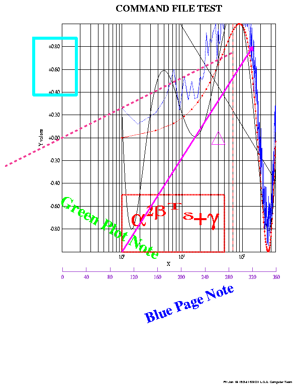
2.4 EXAMPLE
The result in PostScript will
be contained in the file print.ps to be printed or visualized.
Verbose
WindowSize            Width=575       Height=575
Formula               Min=0   Max=360 Npoints=200  Formula="y=sind(x)"
PlotTitle             Title="COMMAND FILE TEST"  Height=1.20
ScaletoFrame
LineJoin              Round
LineStyle             Curve=1  Style=MicroDash  Red   Thickness=2
MarkStyle             Curve=1  Style=BigDot     Size=3
PlottingStep          Curve=1  Step=2

XAxis             Scale=Logarithm   Min=-1   Max=-1
Ytitle            Title="Y values"  Height=1.
Ylimits           Min=-1.  Max=1.0
Ylabel            LabelHeight=1.00   CFormat="%+2.2f"
Rescale

Fit    Function=Polynomial    Curve=1      Npoints=100     Order=6       Mode=Add
Fit    Function=AdvancedFit   Curve=1      Npoints=100     Error=.0001   Mode=Add \
                        Formula="y=a*x+b"       Init="a=3,b=0"
Formula       Npoints=100       Formula="y=y1+rnd()/2"
Extract       File="./data.extract"
PlotText      XStart=32.22%     YStart=81.04%     Color=Red     Style=Bold \
                        Height=3.00     Text="$a^{2$b^{$T}\_{$d}}+$g"
PlotText      XStart=0.11       Ystart=-.5        Color=Green   Style=Bold \
                        Height=2.       Angle=-30     Text="Green Plot Note"
PlotMark      XStart=40.       YStart=0       \
                        Color=Magenta       Style=TriangleUp Size=20
PlotLine      XStart=80%       YStart=0%       XEnd=80%       YEnd=100% \
                        Color=Red       Style=Dash       Thickness=6
PlotBox       XStart=0.       YStart=-1.       XEnd=50.       YEnd=-.5. \
                        Color=Red       Style=MicroDash       Thickness=12
PlotArrow     XStart=0.       YStart=-1        XEnd=150.       YEnd=.8 \
                        Color=Magenta Thickness=10
PlotAxis      Location=Free  \
                        XStart=0.30%   YStart=108.79%  XEnd=100.30%  YEnd=109.16% \
                        Color=Violet        Label=Yes       \
                        Min=0    Max=360   Delta=40 \
                        CFormat="%.0f"  Scale=Linear
PageText      XStart=10.       YStart=25.       Color=Blue      Style=Bold \
                        Angle=20.       Text="Blue Page Note"
PageLine      XStart=0.       YStart=14.       XEnd=16.        YEnd=6. \
                        Color=Plum       Style=Dash       Thickness=.1
PageBox       XStart=2.       YStart=5.       XEnd=5.       YEnd=9. \
                        Color=Cyan       Style=Solid       Thickness=.2
PageArrow     XStart=5.       YStart=8.       XEnd=12.       YEnd=10. \
                        Color=Turquoise       Thickness=.6

DrawCell      XStart=4.       YStart=4.       Width=15.       Height=16. \
                        Type=Color       Mode=ScaleToFrame

SendToFile    File="./print"       Size=15.       Copies=1
 **********************************************************
**********************************************************
A network version of the software (Mgraph_sp ) has been developed; it allows
the visualization of graphics computed in a program. This version is
useful in delicate problems such as the analysis of measurements where the
constraints are: the choice of the sequences to be analyzed and the
adjustment of physical coefficients in a model for example an inversion
and a retrieval of physical parameters.
A library lib_Net_Mgraph.a with various modules to be integrated in the
FORTRAN or C programs has been generated and several examples with comments
are provided with the Mgraph distribution.
This network version makes possible for a user to launch his calculation program on a 1st computer which would run the visualization program Mgraph_sp on a 2nd computer and the graphic result would appear on the X terminal of a 3rd computer. This is possible whatever type of platform is used. (Warning: the user must have a login on the different computers). Usually the 3 steps are launched on the same computer, but this shows the independence of the user's program from the graphic visualization.
| Launch of software (§3.2.1) | run_mgraph |
| run_mgraph_no_display | |
| Global specifications (§3.2.2) | send_resize |
| send_scale_to_frame | |
| send_add_logo | |
| send_signature | |
| Axis drawing (§3.2.3) | send_format |
| send_xaxes2 | |
| send_yaxes2 | |
| send_zaxes2 | |
| send_labelsize | |
| Send of data (§3.2.4) | send_data2 |
| send_data_Xerror | |
| send_data_Yerror | |
| Send of Surface (§3.2.5) | send_datasurf |
| send_irregulardatasurf | |
| send_datasurf3d | |
| send_colorscale | |
| Send of Title or Annotation (§3.2.6) | send_title |
| send_text2 | |
| send_line | |
| send_box | |
| send_mark | |
| The Page Setting (§3.2.7) | send_draw_cell |
| send_page_text | |
| send_page_line | |
| send_page_box | |
| send_page_arrow | |
| The Outputs (§3.2.8) | send_print |
| send_create_ps | |
| send_create_eps | |
| send_export | |
| The Animation (§3.2.9) | send_animate |
| send_clear_window | |
| Close the Dialog (§3.2.10) | send_end_dialog |
| send_exit_mgraph |
In FORTRAN langage, the names of the routines are simply followed of _f.
The detailed description of the parameters of the functions is given below.
The following variables are used in several subroutines.
/*----------------------------------------------------------------------------*/
/* LOGIN          login name; if NULL will be the current login               */
/* SHELL          "rsh" or "remsh"; if NULL will be  "remsh"                  */
/* PATH           path where the program is                                   */
/* PROG           name of the program (Mgraph_sp)                             */
/* COMPUTER       name of the computer where the program have to              */
/*                be launched; if NULL will be server_name                    */
/* DISPLAY        IP Address of terminal                                      */
/*----------------------------------------------------------------------------*/

run_mgraph (client_id, LOGIN, SHELL, PATH, PROG, COMPUTER, DISPLAY);
run_mgraph_no_display (client_id, LOGIN, SHELL, PATH, PROG, COMPUTER, DISPLAY);
int 	client_id;
char 	LOGIN[], SHELL[], PATH[], PROG[], COMPUTER[], DISPLAY[];

call run_mgraph_f (client_id, LOGIN, SHELL, PATH, PROG, COMPUTER, DISPLAY)
call run_mgraph_no_display_f (client_id, LOGIN, SHELL, PATH, PROG, COMPUTER, DISPLAY)
integer 	client_id
character*(*) 	LOGIN, SHELL, PATH, PROG, COMPUTER, DISPLAY
If the file prog.c contains this program, execute the compilation shell:
3.2.2 Global specifications:
The routine ``send_clear_window'' makes it possible to erase the
indicated window. ``send_resize'' makes it possible to redefine the
window geometry. ``send_scale_to_frame'' makes it
possible to limit the axes to truths minimum and maximum whereas
by default an extension of 10% is applied for a better presentation.
``send_add_logo'' and ``send_signature'' make it possible to send a
logo and a signature on the page.
C:
==
send_clear_window(client_id,window);
int         client_id,window;

FORTRAN:
=======
call send_clear_window_f(client_id,window)
integer         client_id,window

/*--------------------------------------------------------------------------------*/
/* width,height            Window size in pixel                                   */
/*--------------------------------------------------------------------------------*/

C:
==
send_resize(client_id,window,width,height);
int 	client_id,window,width,height;

FORTRAN:
=======
call send_resize_f(client_id,window,width,height)
integer 	client_id,window,width,height

/*--------------------------------------------------------------------------------*/
/* flag             0->no    1->yes                                               */
/*--------------------------------------------------------------------------------*/

C:
==
send_scale_to_frame(client_id,window,flag);
int     client_id,window,flag;

FORTRAN:
=======
call send_scale_to_frame_f(client_id,window,flag)
integer     client_id,window,flag

/*--------------------------------------------------------------------------------*/
/* x_position, y_position       position of the logo                              */
/* w_scale, h_scale             scaling    "   "                                  */
/* file_name                    the EPS filename which contains the logo          */
/*--------------------------------------------------------------------------------*/

C:
==
send_add_logo(client_id,x_position,y_position,w_scale,h_scale,file_name);
int     client_id;
float   x_position,y_position,w_scale,h_scale;
char    *file_name;

FORTRAN:
=======
call send_add_logo_f(client_id,x_position,y_position,w_scale,h_scale,file_name)
integer      client_id
real         x_position,y_position,w_scale,h_scale
character    file_name()

/*--------------------------------------------------------------------------------*/
/* signature        your signature                                                */
/*--------------------------------------------------------------------------------*/

C:
==
send_signature(client_id,signature);
int     client_id;
char    *signature;

FORTRAN:
=======
call send_signature_f(client_id,signature)
integer      client_id
character    signature()
3.2.3 Draw axis:
The routine ``send_format'' allows, in only one call, to determine the
axes in X and in Y. The calls of the routines ``send_xaxes2,
send_yaxes2, send_zaxes2 '' make it possible to describe the axes
one by one. ``send_labelsize'' makes it possible to change, in only
one call, the size of all the labels.
/*-------------------------------------------------------------------------------------*/
/*   extend           0=short mode   1=long mode                                       */
/*   XTitle           X Title                                                          */
/*   YTitle           Y Title                                                          */
/*   XForm            X Format  the C format formulation   ("%.2f" for ex.)            */
/*   YForm            Y Format    "    "        "                                      */
/*   Xsize            X Label size                                                     */
/*   Ysize            Y Label size                                                     */
/*   Xgrid            Grid type (10=grid 11=halftone 12=nogrid)                        */
/*   Xlab             0=Draw label on X (1=NoXlabel)                                   */
/*   Ygrid            Grid type (10=grid 11=halftone 12=nogrid)                        */
/*   Ylab             0=Draw label on Y (1=NoYlabel)                                   */
/*   Xlog             X log if =1                                                      */
/*   Ylog             Y log if =1                                                      */
/*   Xstep            X Step (if = 0 no small ticks)                                   */
/*   Ystep            Y Step                                                           */

/*  if extend = 1 (long mode):                                                         */
/*   Xmin, Xmax       X limits                                                         */
/*   Xref             X Reference value                                                */
/*   Xtick            X tick nb                                                        */
/*   Ymin, Ymax       Y limits                                                         */
/*   Yref             Y Reference value                                                */
/*   Ytick            Y tick nb                                                        */
/*-------------------------------------------------------------------------------------*/

C:
==
send_format(client_id,window,extend,XTitle,YTitle,XForm,YForm,Xsize,Ysize,
      Xgrid,Xlab,Ygrid,Ylab,Xlog,Ylog,Xstep,Ystep,
      Xmin,Xmax,Xref,Xtick,Ymin,Ymax,Yref,Ytick);

int         client_id,window,extend;
char        *XTitle,*YTitle ,*XForm,*YForm;
float       Xsize,Ysize;
int         Xgrid,Xlab,Ygrid,Ylab,Xlog,Ylog;
float       Xstep,Ystep;
float       Xmin,Xmax,Xref;
int         Xtick;
float       Ymin,Ymax,Yref;
int         Ytick;

FORTRAN:
=======
call send_format_f(client_id,window,extend,XTitle,YTitle,XForm,YForm,Xsize,Ysize,
      Xgrid,Xlab,Ygrid,Ylab,Xlog,Ylog,Xstep,Ystep,
      Xmin,Xmax,Xref,Xtick,Ymin,Ymax,Yref,Ytick)

integer     client_id,window,extend
character   XTitle(),YTitle(),XForm(),YForm()
real        Xsize,Ysize
integer     Xgrid,Xlab,Ygrid,Ylab,Xlog,Ylog
real        Xstep,Ystep
real        Xmin,Xmax,Xref
integer     Xtick
real        Ymin,Ymax,Yref
integer     Ytick


/*--------------------------------------------------------------------------------------*/
/* legend               The text which is displayed under the axis                      */
/* format               the C format formulation   ("%.2f" for ex.)                     */
/* label size           factor on label size                                            */
/* min, max             the limits of axis (-1 : uses the best)                         */
/* grid                 10= grid 11= half tone 12= no grid                              */
/* thickness            line factor                                                     */
/* rotation             label text rotation in degrees                                  */
/* step                 the step in your units between two ticks (-1:uses the best)     */
/* ref                  reference value   (-1 : uses the best)                          */
/* tick                 step (in ticks) between two labeled ticks  (-1 : uses the best) */
/* log                  0=linear 1=logarithm  2=formula 3=time  4=degree                */
/* Formula              (if log = 2)                                                    */
/*--------------------------------------------------------------------------------------*/

C:
==
send_xaxes2(client_id,window,legend,format,label_size,min,max,grid,
            color,thickness,rotation,step,ref,tick,log,Formula);
send_yaxes2(client_id,window,legend,format,label_size,min,max,grid,
            color,thickness,rotation,step,ref,tick,log,Formula);
send_zaxes2(client_id,window,legend,format,label_size,min,max,grid,
            color,thickness,rotation,step,ref,tick,log,Formula);

int         client_id,window;
char        *legend,*format;
float       label_size,min,max;
int         grid,color,thickness;
float       rotation,step,ref;
int         tick,log;
char        *Formula;

FORTRAN:
=======
call send_xaxes2_f(client_id,window,legend,format,label_size,min,max,grid,
            color,thickness,rotation,step,ref,tick,log,Formula)
call send_yaxes2_f(client_id,window,legend,format,label_size,min,max,grid,
            color,thickness,rotation,step,ref,tick,log,Formula)
call send_zaxes2_f(client_id,window,legend,format,label_size,min,max,grid,
            color,thickness,rotation,step,ref,tick,log,Formula)

integer       client_id,window;
character*(*) legend,format;
real          label_size,min,max;
integer       grid,color,thickness;
real          rotation,step,ref;
integer       tick,log;
character*(*) Formula;


/*-----------------------------------------------------------------------------*/
/* tit            size of title                                                */
/* xlab           size of Xaxis labels                                         */
/* ylab           size of Yaxis labels                                         */
/* xtit           size of Xaxis title                                          */
/* ytit           size of Yaxis title                                          */
/*-----------------------------------------------------------------------------*/

C:
==
send_labelsize(client_id,window,tit,xlab,ylab,xtit,ytit);
int         client_id,window;
float       tit,xlab,ylab,xtit,ytit;

FORTRAN:
=======
call send_labelsize_f(client_id,window,tit,xlab,ylab,xtit,ytit)
integer     client_id,window
real        tit,xlab,ylab,xtit,ytit
3.2.4 Send data to Mgraph:
The routine ``send_data2 '' makes it possible to send in a window a
set of data, in 2 arrays (X and Y). the routines
``send_data_Xerror'' and ``send_data_Yerror'' makes it possible to
draw these data with a bar of error (X, Y and array ERROR). For
each one of these calls, you can determine the number of the curve
(-1 will number automatically), the style (color, line and type of
marker) of the curve (and of the bars of error).
/*----------------------------------------------------------------------------*/
/* clear               Window have to be cleared ? (Bool)                     */
/* plot_nb (0->512)    Number of the plot (-1 will determine an available one */
/* nbp                 Number of points in the data                           */
/* xx                  x       data                                           */
/* yy                  f(x)    data                                           */
/* error               X or Y error bar (Y+err Y-err (or X+err X-err) will be drawn) */
/*----------------------------------------------------------------------------*/

C:
==
send_data2(client_id,window,clear,plot_nb,nbp,xx,yy,color,style,mark,thickness,marksize);

int      client_id;
int      window,clear,plot_nb, nbp;
float    *xx,*yy;
int      color,style,mark,thickness,marksize;

send_data_Xerror(client_id,window,clear,plot_nb,nbp,xx,yy,error,
                bar_color,bar_style,bar_mark,bar_thickness,bar_marksize,
                curve_color,curve_style,curve_mark_type,curve_line_thickness,curve_mark_size);
send_data_Yerror(client_id,window,clear,plot_nb,nbp,xx,yy,error,
                bar_color,bar_style,bar_mark,bar_thickness,bar_marksize,
                curve_color,curve_style,curve_mark_type,curve_line_thickness,curve_mark_size);

int      client_id,window,clear,plot_nb,nbp;
float    *xx,*yy,*error;
int      bar_color,bar_style,bar_mark,bar_thickness,bar_marksize;
int      curve_color,curve_style,curve_mark_type,curve_line_thickness,curve_mark_size;

FORTRAN:
=======
call send_data2_f(client_id,window,clear,plot_nb,nbp,xx,yy,color,style,mark,thickness,marksize)

integer      client_id
integer      window,clear,plot_nb, nbp
real         xx(nbp),yy(nbp)
integer      color,style,mark,thickness,marksize

call send_data_Xerror_f(client_id,window,clear,plot_nb,nbp,xx,yy,error,
                bar_color,bar_style,bar_mark,bar_thickness,bar_marksize,
                curve_color,curve_style,curve_mark_type,curve_line_thickness,curve_mark_size)
call send_data_Yerror_f(client_id,window,clear,plot_nb,nbp,xx,yy,error,
                bar_color,bar_style,bar_mark,bar_thickness,bar_marksize,
                curve_color,curve_style,curve_mark_type,curve_line_thickness,curve_mark_size)

integer      client_id,window,clear,plot_nb,nbp
real         xx(nbp),yy(nbp),error(nbp)
integer      bar_color,bar_style,bar_mark,bar_thickness,bar_marksize
integer      curve_color,curve_style,curve_mark_type,curve_line_thickness,curve_mark_size
3.2.5 Send a surface to Mgraph:
The routine ``send_datasurf'' makes it possible to send a surface,
in a regular grid, to Mgraph. The points are arranged in 1 array
(data). ``send_irregulardatasurf'' makes it possible to send an
irregular surface in 3 arrays (XX, YY and ZZ). ``send_datasurf3d''
allows a representation 3D of the surface previously drawn in a
window and the call of ``send_colorscale'' makes it possible to draw
a scale color, linear or using squares.
For the description of the internal color scale, to see the §1.2.8.
/*-----------------------------------------------------------------------------------*/
/* width, height       surface dimensions                                            */
/* xmin xmax ymin ymax limits on X and Y                                             */
/* data[width*height]  data values                                                   */
/* nbcont              number of contour values                                      */
/* cont[nbcont]        contour values                                                */
/* color[nbcont]       (0->12 - 16)                                                  */
/* style[nbcont]       (0->7)      Line style                                        */
/* mark[nbcont]        (0->15)     Mark type                                         */
/* dolabel[nbcont]     Draw label? 0=No 1=Yes                                        */
/* add[4]              Surface , Region , Dots , Triangles (0/1)                     */
/* undef               Undef value (float)                                           */
/* distance            Region distance factor                                        */
/* pix[4]              Color tranformation: minv maxv minp maxp                      */
/* nlut                0=no lut   1->14=internal LUT 256=use following LUTS          */
/* Red[256]            LUT                                                           */
/* Green[256]          LUT                                                           */
/* Blue[256]           LUT                                                           */
/* near                pixel interpolation: 0=No 1=Yes                               */
/* Format              label C format                                                */
/* AddMode             1 = add contours on graphic window                            */
/*-----------------------------------------------------------------------------------*/

C:
==
send_datasurf(client_id,window,width,height,xmin,xmax,ymin,ymax,data,nbcont,cont,
              color, style,mark ,dolabel,add,undef,distance,pix,nlut,
              red,green,blue,near,Format,AddMode);
int        client_id,window,width,height;
float      xmin,xmax,ymin,ymax;
float      *data;
int        nbcont;
float      *cont;
int        *color,*style,*mark,*dolabel;
int        *add;
float      undef,distance,*pix;
int        nlut;
short      *red,*green,*blue;
int        near;
char       *Format;
int        AddMode;

FORTRAN:
=======
call send_datasurf_f(client_id,window,width,height,xmin,xmax,ymin,ymax,data,nbcont,cont,
              color, style,mark ,dolabel,add,undef,distance,pix,nlut,
              red,green,blue,near,Format,AddMode)
integer        client_id,window,width,height
real        xmin,xmax,ymin,ymax
real        data(nbp)
integer     nbcont
real        cont(nbcont)
integer     color(nbcont),style(nbcont),mark(nbcont),dolabel(nbcont)
integer     add(4)
real        undef,distance,pix(4)
integer     nlut
integer*2   red(256),green(256),blue(256)
integer     near
character*(*)  Format
integer     AddMode


/*-----------------------------------------------------------------------------------*/
/* width, height       surface dimensions [default 0]                                */
/* size                size of matrix X,Y,Z                                          */
/* xx                  X values (float)                                              */
/* yy                  Y values (float)                                              */
/* zz                  Z values (float)                                              */
/*-----------------------------------------------------------------------------------*/

C:
==
send_irregulardatasurf(client_id,window,width,height,size,xx,yy,zz,nbcont,cont,
		color,style,mark,dolabel,add,undef,distance,pix,nlut,
		red,green,blue,near,Format,AddMode);

int        client_id,window,width,height,size;
float      *xx,*yy,*zz;
int        nbcont;
float      *cont;
int        *color,*style,*mark,*dolabel;
int        *add;
float      undef,distance,*pix;
int        nlut;
short      *red,*green,*blue;
int        near;
char       *Format;
int        AddMode;

FORTRAN:
=======
call send_irregulardatasurf(client_id,window,width,height,size,xx,yy,zz,nbcont,cont,
		color,style,mark,dolabel,add,undef,distance,pix,nlut,
		red,green,blue,near,Format,AddMode)

integer        client_id,window,width,height,size
real           xx(size),yy(size),zz(size)
integer        nbcont
real           cont(nbcont)
integer        color(nbcont),style(nbcont),mark(nbcont),dolabel(nbcont)
integer        add(4)
real           undef,distance,pix(4)
integer        nlut
integer*2      red(256),green(256),blue(256)
integer        near
character*(*)  Format
integer        AddMode

/*-----------------------------------------------------------------------------------*/
/* updown              Up/Down angle in degrees                                      */
/* rightleft           Right/Left angle in degrees                                   */
/* groundlevel         Undef=8421                                                    */
/* stretch             between  0 to 1 : reduces z impact                            */
/* zeroposition        between -1 to 1 : shifts the graph position                   */
/* addings3D[8]        Top surface, Bottom surface, Surface, Grids,                  */
/*                     Top curves, Bottom curves  (0/1)     (7 &  8 unused)          */
/* nbgrid              Number of grids                                               */
/* thickness	       Grid thickness                                                */
/* color               Grid color (0->12 or 16 for white)                            */
/*-----------------------------------------------------------------------------------*/

C:
==
send_datasurf3d(client_id,window,updown,rightleft,groundlevel,
                stretch,zeroposition,addings3D,nbgrid,thickness,color);

int         client_id,window;
float       updown,rightleft,groundlevel,stretch,zeroposition;
int         *addings3D,nbgrid,thickness,color;

FORTRAN:
=======
call send_datasurf3d(client_id,window,updown,rightleft,groundlevel,
                stretch,zeroposition,addings3D,nbgrid,thickness,color)

integer         client_id,window
real            updown,rightleft,groundlevel,stretch,zeroposition
integer         addings3D(8),nbgrid,thickness,color


/*-----------------------------------------------------------------------------------*/
/* mode                0=linear  1=boxes                                             */
/* x1,y1,x2,y2         color scale positions                                         */
/* min,max             color scale stretch: 0->255                                   */
/* position            0=Down/Right  1=Up/Left                                       */
/* color_label         Label color (0->12 or 16 for white)                           */
/* NoTick              0=tick  1=no tick                                             */
/* size_label          the size label factor                                         */
/* coord               0=percentage   1=user units                                   */
/* format              the C format formulation   ("%.2f" for ex.)                   */
/* list                list of pixel value followed by a value or a label            */
/*-----------------------------------------------------------------------------------*/

C:
==
send_colorscale(client_id,window,mode,x1,y1,x2,y2,min,max,position,color_label,
		NoTick,size_label,coord,format,list);

int         client_id,window,mode;
float       x1,y1,x2,y2;
int         min,max,position,color_label,NoTick;
float       size_label;
int         coord;
char        *format,*list;

FORTRAN:
=======
call send_colorscale(client_id,window,mode,x1,y1,x2,y2,min,max,position,color_label,
		NoTick,size_label,coord,format,list)

integer         client_id,window,mode
real            x1,y1,x2,y2
integer         min,max,position,color_label,NoTick
real            size_label
integer         coord
character*(*)   format,list
3.2.6 Send the title or an annotation to Mgraph:
The following calls enable you to add a title in a window or
annotations: text, line or mark. The variable ``relative'' makes it possible
to attach the annotations to the graph in real coordinates or to attach
them to the graph itself (in %).
/*----------------------------------------------------------------------------*/
/* text                      the text which is to be shown                    */
/* x_position, y_position    position of the text (or marker)                 */
/* x_start,y_start           start position of the line (or box)              */
/* x_end,y_end               end position of the line (or box)                */
/* rotation                  rotation angle in degree                         */
/* size                      factor                                           */
/* bold                      0->plain text  1->bold text                      */
/* thickness                 Line thickness factor                            */
/* relative                  0->relative to frame in %  1-> user coordinates  */
/*----------------------------------------------------------------------------*/

C:
==
send_title(client_id,window,text);
int 	client_id,window;
char 	*text;

send_text2(client_id,window,color,rotation,size,bold,x_position,y_position,text,relative);
int         client_id,window,color;
float       rotation,size;
int         bold;
float       x_position,y_position;
char        *text;
int         relative;

send_line(client_id,window,color,style,thickness,x_start,y_start,x_end,y_end,relative);
int         client_id,window,color,style,thickness;
float       x_start,y_start,x_end,y_end;
int         relative;

send_box(client_id,window,color,style,thickness,x_start,y_start,x_end,y_end,relative);
int        client_id,window,color,style,thickness;
float      x_start,y_start,x_end,y_end;
int        relative;

send_mark(client_id,window,color,type,size,x_pos,y_pos,relative);
int        client_id,window,color,type,size;
float      x_pos,y_pos;
int        relative;


FORTRAN:
=======
call send_title_f(client_id,window,text)
integer 	client_id,window
character*(*)  	text

call send_text2_f(client_id,window,color,rotation,size,bold,x_position,y_position,text,relative)
integer         client_id,window,color
real            rotation,size
integer         bold
real            x_position,y_position
character*(*)   text
integer         relative

call send_line_f(client_id,window,color,style,thickness,x_start,y_start,x_end,y_end,relative)
integer         client_id,window,color,style,thickness
real            x_start,y_start,x_end,y_end
integer         relative

call send_box_f(client_id,window,color,style,thickness,x_start,y_start,x_end,y_end,relative)
integer        client_id,window,color,style,thickness
real           x_start,y_start,x_end,y_end
integer        relative

call send_mark_f(client_id,window,color,type,size,x_pos,y_pos,relative)
integer        client_id,window,color,type,size
real           x_pos,y_pos
integer        relative
3.2.7 Make a page setting
You can print your graph directly by using outputs PostScript, GIF or
Tiff but also by making a page setting with the following calls:
``send_draw_cell'' makes it possible to send the graph in a cell
positioned on a page, then ``send_page_text'' etc... makes it
possible to make annotations on the page.
/*------------------------------------------------------------------------------------*/
/* x_position, y_position    position of the cell on the page   in cm                 */
/* width, height             size in cm                                               */
/* type                      0=B/W    1=GreyScale    2=Color                          */
/* orientation               0=Portrait 1=Landscape                                   */
/* fit_frame                 fit the frame? 0=No     1=Yes                            */
/*------------------------------------------------------------------------------------*/

C:
==
send_draw_cell(client_id,window,x_position,y_position,width,height,type,orientation,fit_frame);
int        client_id,window;
float      x_position,y_position,width,height;
int        type,orientation,fit_frame;

FORTRAN:
=======
call send_draw_cell_f(client_id,window,x_position,y_position,width,height,type,orientation,fit_frame)
integer        client_id,window
real           x_position,y_position,width,height
integer        type,orientation,fit_frame;

/*-------------------------------------------------------------------------------------*/
/* x_position, y_position    position of the text on the page   in cm                  */
/* bold                bold text? 0=No     1=Yes                                       */
/* height              text height in cm                                               */
/* rotation            text rotation in degrees                                        */
/* text                the text which is to be shown                                   */
/* x_start, y_start    start position of the line (box, arrow) in cm                   */
/* x_end, y_end        end  position of the line (box, arrow) in cm                    */
/* thickness           Line thickness in cm                                            */
/*-------------------------------------------------------------------------------------*/

C:
==
send_page_text(client_id,x_position,y_position,color,bold,height,rotation,text);
int         client_id;
float       x_position,y_position;
int         color,bold;
float       height,rotation;
char        *text;

send_page_line(client_id,x_start,y_start,x_end,y_end,color,style,thickness);
int         client_id;
float       x_start,y_start,x_end,y_end;
int         color,style;
float       thickness;

send_page_box(client_id,x_start,y_start,x_end,y_end,color,style,thickness);
int         client_id;
float       x_start,y_start,x_end,y_end;
int         color,style;
float       thickness;

send_page_arrow(client_id,x_start,y_start,x_end,y_end,color,style,thickness);
int         client_id;
float       x_start,y_start,x_end,y_end;
int         color,style;
float       thickness;

FORTRAN:
=======
call send_page_text_f(client_id,x_position,y_position,color,bold,height,rotation,text)
integer          client_id
real             x_position,y_position
integer          color,bold
real             height,rotation
character*(*)    text

call send_page_line_f(client_id,x_start,y_start,x_end,y_end,color,style,thickness)
integer         client_id
real            x_start,y_start,x_end,y_end
integer         color,style
real            thickness

call send_page_box_f(client_id,x_start,y_start,x_end,y_end,color,style,thickness)
integer         client_id
real            x_start,y_start,x_end,y_end
integer         color,style
real            thickness

call send_page_arrow_f(client_id,x_start,y_start,x_end,y_end,color,style,thickness)
integer         client_id
real            x_start,y_start,x_end,y_end
integer         color,style
real            thickness
3.2.8 The outputs:PostScript, Gif or Tiff
You can print your graph or your page setting either directly on a
printer through a command ``shell'', or in a file (PS or EPS). You can
also export a graph in a file Tiff or GIF.
/*------------------------------------------------------------------------------------*/
/*           allows you to send the graphic window  to a spooler command              */
/*              or in a  (Encapsulated)PostScript file                                */
/* size                 size in cm (std 16 cm)                                        */
/* type                 0=B/W    1=GreyScale    2=Color                               */
/* square               square frame? 0=No     1=Yes                                  */
/* logo                 add the logo? 0=No     1=Yes                                  */
/* orientation          0=Portrait 1=Landscape                                        */
/* printer_shell        spooler command: example: "lp -d Myprinter"                   */
/* file_name            your PS file name                                             */
/*------------------------------------------------------------------------------------*/

C:
==
send_print(client_id,window,size,type,square,logo,orientation,printer_shell);
int        client_id,window;
float      size;
int        type,square,logo,orientation;
char       *printer_shell;

send_create_ps (client_id,window,size,type,square,logo,orientation,file_name);
int     client_id,window;
float   size;
int     type,square,logo,orientation;
char    *file_name;

send_create_eps(client_id,window,type,orientation,file_name);
int     client_id,window,type,orientation;
char    *file_name;

FORTRAN:
=======
call send_print_f(client_id,window,size,type,square,logo,orientation,printer_shell)
integer        client_id,window
real           size
integer        type,square,logo,orientation
character*(*)  printer_shell

call send_create_ps_f(client_id,window,size,type,square,logo,orientation,file_name)
integer        client_id,window
real           size
integer        type,square,logo,orientation
character*(*)  file_name

call send_create_eps_f(client_id,window,type,orientation,file_name)
integer        client_id,window,type,orientation
character*(*)  file_name

/*------------------------------------------------------------------------------------*/
/*           allows you to export the graphic window                                  */
/*                   in a Gif / Tiff file                                             */
/* type                 0-> gif 1-> Tiff                                              */
/* file_name            your Gif/Tiff file name                                       */
/*------------------------------------------------------------------------------------*/

C:
==
send_export(client_id,window,type,file_name);
int     client_id,window;
int     type;
char    *file_name;

FORTRAN:
=======
call send_export_f(client_id,window,type,file_name)
integer          client_id,window
integer          type
character*(*)    file_name
3.2.9 Animate curves:
If several curves were plotted in the window, they can be animated
in the following way:
/*-------------------------------------------------------------*/
/* elapse               time : 10 -> 100                       */
/* plot step            > 1 if the animation is too slow       */
/*-------------------------------------------------------------*/

C:
==
send_animate(client_id,window,elapse,plot_step)
int          client_id,window,elapse,plot_step;

FORTRAN:
=======
call send_animate_f(client_id,window,elapse,plot_step)
integer        client_id,window,elapse,plot_step
3.2.10 Close the session:
The routine ``send_end_dialog'' makes it possible to leave your
program by preserving active Mgraph. The routine
``send_exit_mgraph'' leaves Mgraph.
C:
==
send_end_dialog(client_id)
int      client_id;

send_exit_mgraph(client_id)
int      client_id;

FORTRAN:
=======
call send_end_dialog_f(client_id)
integer      client_id

call send_exit_mgraph_f(client_id)
integer      client_id
3.3 C program examples:
/*-----------------------------------------------
        SHORT PROGRAM:
        You just need 3 calls to draw a curve:
        run_mgraph:       Calling of the software
        send_data2:       Drawing of 4 curves (sin) into 4 windows
        send_end_dialog:  Close Dialog: Mgraph remains active
------------------------------------------------*/

#include <stdio.h>
#include <math.h>

#define FALSE 0
#define TRUE  1

#define LOGIN ""
#define SHELL "remsh"
#define PATH "/usr/local/bin"
#define PROG "Mgraph_sp"
#define COMPUTER ""
#define DISPLAY ""

extern int run_mgraph();
main()
{
int mgraph_no=1,nbp = 512,id;
float *xx,*yy;
int i,plot_no;

/*========================================================================================
 START MGRAPH_SP MODULE: run_mgraph
        LOGIN:  login name;             if NULL will be the current login
        SHELL:  "rsh" or "remsh";       if NULL will be  "remsh"
        PATH :  path where the program is
        PROG :  name of the program (Mgraph_sp)
        COMPUTER:       name of the computer where the program has to
                        be launched;    if NULL will be the server name
        DISPLAY: Your Display Id;       if NULL will be your DISPLAY address
                                             from your environment
==========================================================================================*/

        if(!run_mgraph(mgraph_no,LOGIN,SHELL,PATH,PROG,COMPUTER,DISPLAY))
        {
                printf("Cannot start Mgraph\n");
                exit(0);
        }

        xx = (float *) malloc( sizeof(float) * nbp );
        yy = (float *) malloc( sizeof(float) * nbp );

        for (plot_no=1;plot_no<5;plot_no++){
        id = plot_no;

            for(i=0;i<nbp;i++){
                xx[i] = i * 3.141592 * plot_no / nbp;
                yy[i] = sin((double)xx[i]) / plot_no;
            }
/*-----------------------------------------------
SEND DATA ON WINDOW
send_data2(client_id,window,clear,plot_nb,nbp,$\times$,yy,color,style,mark,thickness,marksize);

   id    : Number of window (from 1 to 5)
   0     : window will not be cleared
   -1    : number of the plot
   nbp   : Number of points in xx and yy arrays
  xx,yy  : data arrays
  plot_no: color of the curve
  0      : line style (0=solid)
  0      : mark style (0=no mark)
  1      : line thickness
  0      : mark size
------------------------------------------------*/
            send_data2(mgraph_no,id,0,-1,nbp,xx,yy,plot_no,0,0,1,0);
        }

        send_end_dialog(mgraph_no);
        free(xx);
        free(yy);
}
/*-----------------------------------------------
   RELATED PROGRAM: drawing with interaction between software and Mgraph
  -----------------------------------------------
  COMMON VARIABLES:
     int Mgraph_no Sequence number of the software;
                      several Mgraph can be launched at the same time id (several Mgraph can be launched)
     int nwindow   Number of window in which the data will be shown (-1=Current)
     int color     Number of the color: from 0 to 12:
                          Red, Blue, Magenta, Black, Green, Forest, Sienna,
                          Yellow, Coral, Violet, Plum, Cyan, Turquoise
			  Plum, Cyan,Turquoise
                      and 16 for the White
     int linestyle Style of the line: from 0 to 7:
                          Solid, NoLine, MicroDash, SmallDash,
                         Dash, LongDash, DashDot, LineDot
     int marker    Style of the marker: from 0 to 15:
                          NoMark, BigDot, SmallDot, Cross, X, Square,
                          Diamond, TriangleUp, TriangleDown, Circle
                          filled: Square, Diamond, TriangleUp, TriangleDown, Circle
-----------------------------------------------*/

#include <stdio.h>
#include <math.h>
#include <unistd.h>

#define FALSE 0
#define TRUE  1

#define LOGIN NULL
#define SHELL NULL
#define PATH "/usr/local/bin"
#define PROG "Mgraph_sp"
#define COMPUTER ""
#define DISPLAY NULL
#define XFormula "cos(x)"
#define YFormula NULL

extern int run_mgraph();
main()
{
float *xx,*yy;
int   i,nbp,plot_no;
float  coef;

int   Mgraph_no;
int   nwindow;
int   width;
int   height;
char  title[128],texte[128];
char  TitleAxis[128];
char  Format[128];
float xmin,xmax,ymin,ymax;
int   grid;
float xstep,ystep;
float xbase,ybase;
int   ixtic,iytic;
int   ixlog,iylog;
int   clear,color,linestyle,marker;
float posx,posy;


	clear = 0;
	color = 0;
	linestyle = 0;
	marker = 0;
	posy=0.1;

/*========================================================================================
 START MGRAPH_SP MODULE: run_mgraph
        LOGIN:  login name; 		if NULL will be the current login
        SHELL:  "rsh" or "remsh"; 	if NULL will be  "remsh"
        PATH :  path where the program is
        PROG :  name of the program (Mgraph_sp)
        COMPUTER:       name of the computer where the program has to
                        be launched; 	if NULL will be the server name
	DISPLAY: Your Display Id; 	if NULL will be your DISPLAY address
                                             from your environment
==========================================================================================*/

        Mgraph_no = 1;
	if(!run_mgraph(Mgraph_no,LOGIN,SHELL,PATH,PROG,COMPUTER,DISPLAY))
	{
		printf("Cannot start Mgraph\n");
		exit(0);
	}

	nbp = 512;
	xx = (float *) malloc( sizeof(float) * nbp );
	yy = (float *) malloc( sizeof(float) * nbp );

/*========================================================================================
SEND_RESIZE WINDOW
	int width,height      = window size  in pixel
==========================================================================================*/

	width=600;
	height=500;
	nwindow = 1;
	send_resize(Mgraph_no,nwindow,width,height);

/*=========================================================================================
SEND TITLE
	char title[] = the text which is to be shown
==========================================================================================*/

	strcpy(title,"y=sin(x) Window 1");
	send_title(Mgraph_no,nwindow,title);

/*=========================================================================================
SEND AXES
send_xaxes2(client_id,window,legend,format,label_size,min,max,grid,
            color,thickness,rotation,step,ref,tick,log,Formula);

	CAREFUL with types !!!
      char  legend               The text which is displayed under the axis
      char  format               the C format formulation   ("%.2f" for ex.)
      float label size           factor on label size
      float min,max              the limits of axis (-1 : uses the best)
      int   grid                 10= grid 11= half tone 12= no grid
      int   color                color type (3=black)
      int   thickness            thickness of the line factor
      float rotation             label text rotation in degrees
      float step                 the step in your units between two ticks (-1:uses the best)
      float ref                  reference value   (-1 : uses the best)
      int   tick                 step (in ticks) between two labeled ticks  (-1 : uses the best)
      int   log                  0=linear 1=logarithm  2=formula 3=time  4=degree
      char  Formula[]            (if log = 2)
============================================================================================*/

      xmin = 0.;
      xmax = 3.15;
      xstep= -1.;
      xbase= -1.;
      grid= 12;
      ixtic= -1;
      ixlog=  2;

 	send_xaxes2(Mgraph_no,nwindow,"0 <angle< $p","%.2f",1.0,
			xmin,xmax,grid,3,1,30.0,xstep,xbase,ixtic,ixlog,XFormula);

      ymin = 0.;
      ymax = 10.;
      ystep= -1.;
      ybase= -1.;
      iytic= -1;
      iylog=  0;

	send_yaxes2(Mgraph_no,nwindow,"computed sinus","%.2f",1.0,
			ymin,ymax,grid,3,1,30.0,ystep,ybase,iytic,iylog,YFormula);

	coef = 1.;

	for(plot_no=1;plot_no<5;plot_no++){

/*=======================================================================================
	Compute data...
=========================================================================================*/

	    for(i=0;i<nbp;i++){
	        xx[i] = (float)i * 3.141592 / nbp;
	        yy[i] = coef * sin((double)xx[i]) ;
	    }

/*========================================================================================
 SEND DATA ON WINDOW nwindow
send_data2(client_id,window,clear,plot_nb,nbp,xx,yy,color,style,mark,thickness,marksize);

     int plot_nb      Number of the curve (-1 will determine an available one)
     int nbp          Number of points in the data
     float xx         x    data
     float yy         f(x) data
     int color
     int style
     int mark
     int thickness
     int marksize
========================================================================================*/

	    send_data2(Mgraph_no,nwindow,clear,plot_no,nbp,xx,yy,color,linestyle,marker,1,1);

/*===========================================================================================
ADD TEXT ON WINDOW
        send_text2(client_id,window,color,rotation,size,bold,x_pos,y_pos,text,relative);
   float rotation       rotation angle in degree
   float size           factor size of the text
   int   bold           0->plain text  1->bold text
   float x_pos,y_pos    position of the marker (or the text)
   char  text           the text which is to be shown
   int   relative       0->relative to frame in % 1->relative to real coordinates
===========================================================================================*/

	    posx = 80;
	    sprintf(texte,"%.5f %c",3.141592 * plot_no,0);
	    send_text2(Mgraph_no,nwindow,color,0.0,1.,0,posx,posy,texte,0);
	    color++;
	    if (color>12) color = 0;
	    posy += 5;
	    printf("You can adjust your curve in your program\n");
            printf("enter new coef (between 1-10) for a new curve: ");
	    scanf("%g",&coef);
	}

/*====================================================================================
ANIMATE PLOTS
	int elapse_time   10 -> 100
	int step    > 1 if the animation is too slow
======================================================================================*/

	send_animate(Mgraph_no,nwindow,100,1);
	printf("Touch the plot Window 1 to animate.... \n");

/*====================================================================================
 	New Window, same Mgraph,  with the cosinus...
======================================================================================*/
      nwindow = 2;
      strcpy(title,"y=cos(x) Window 2");
      send_title(Mgraph_no,nwindow,title);

      send_xaxes2(Mgraph_no,nwindow,"Angle","%.1f",1.0,0.,10.,11,3,1,30.0,-1.,5.,2,4,XFormula);
      send_yaxes2(Mgraph_no,nwindow,"cos(x)","%.2f",1.0,-1.,-1.,11,3,1,30.0,ystep,ybase,2,0,YFormula);

      color=0;
      clear=1;
      linestyle=2;

      for(plot_no=0; plot_no<5; plot_no++){
         for(i=0;i<nbp;i++){
            *(xx+i) = i * 3.141592 * plot_no / nbp;
            *(yy+i) = cos(*(xx+i))* plot_no/10.;
         }
          send_data2(Mgraph_no,nwindow,clear,-1,nbp,xx,yy,color,linestyle,marker,1,1);
          color++;
          linestyle++;
          clear=0;
      }


/*===========================================================================================
EXIT_MAIN_PROGRAM
	before quitting your main program,  call send_end_dialog
	to keep Mgraph running
===========================================================================================*/

	send_end_dialog(Mgraph_no);
	free(xx);
	free(yy);
}
c==================================================================
c       SHORT PROGRAM:
c       You just need 3 calls to draw a curve:
c       run_mgraph:       Calling of the software
c       send_data2:       Drawing of 1 curve (sin)
c       send_end_dialog:  Close Dialog: Mgraph remains active
c==================================================================
      CHARACTER*(*) PROG,PATH
      PARAMETER (PATH ='/usr/local/bin/')
      PARAMETER (PROG ='Mgraph_sp')

      real xx(512),yy(512)
      nbp =512
      Mgraph_no = 1
      nwindow = -1
C========================================================================================
c START MGRAPH_SP MODULE: run_mgraph_f
c        LOGIN:  login name;             if NULL will be the current login
c        SHELL:  "rsh" or "remsh";       if NULL will be  "remsh"
c        PATH :  path where the program is
c        PROG :  name of the program (Mgraph_sp)
c        COMPUTER:       name of the computer where the program has to
c                        be launched;    if NULL will be the server name
c        DISPLAY: Your Display Id;       if NULL will be your DISPLAY address
c                                             from your environment
C========================================================================================

      call run_mgraph_f(Mgraph_no," "," ",PATH,PROG," "," ")
c
c Compute the data
c
      do i = 1,nbp
            xx(i) = i * 3.141592 /nbp
            yy(i) = sin(xx(i))
      enddo
c-----------------------------------------------
c   nwindow    : Number of window
c   1     : window will be cleared
c   1     : number of the plot
c   nbp   : Number of points in xx and yy arrays
c  xx,yy  : data arrays
c   1     : color of the curve (1=blue)
c   0     : line style (0=solid)
c   4     : mark style (4=square)
c   1     : line thickness
c   1     : mark size
c------------------------------------------------*/
      call send_data2_f(Mgraph_no,nwindow,1,1,nbp,xx,yy,1,0,4,1,1)

c===========================================================================================
c EXIT_MAIN_PROGRAM
c       before quitting your main program,  call send_end_dialog
c       to keep Mgraph running
c===========================================================================================

      call send_end_dialog_f(Mgraph_no)
      stop
      end
c-----------------------------------------------
c  RELATED PROGRAM: drawing with interaction between software and Mgraph
c -----------------------------------------------
c COMMON VARIABLES:
c    integer Mgraph_no Sequence number of the software;
c                        several Mgraph can be launched at the same time id (several Mgraph can be launched)
c    integer nwindow   Number of window in which the data will be shown (-1=Current)
c    integer color     Number of the color: from 0 to 12:
c                         Red, Blue, Magenta, Black, Green, Forest, Sienna,
c                         Yellow, Coral, Violet, Plum, Cyan, Turquoise
c                         Plum, Cyan,Turquoise
c                        and 16 for the White
c    integer linestyle Style of the line: from 0 to 7:
c                         Solid, NoLine, MicroDash, SmallDash,
c                           Dash, LongDash, DashDot, LineDot
c    integer marker    Style of the marker: from 0 to 15:
c                         NoMark, BigDot, SmallDot, Cross, X, Square,
c                         Diamond, TriangleUp, TriangleDown, Circle
c                         filled: Square, Diamond, TriangleUp, TriangleDown, Circle
c-----------------------------------------------


      CHARACTER*(*) LOGIN,SHELL,PROG,PATH,COMPUTER
      CHARACTER*(*) X_FORMULA,Y_FORMULA,DISPLAY
      PARAMETER (LOGIN=" ")
      PARAMETER (SHELL=" ")
      PARAMETER (PATH ="//usr/local/bin/")
      PARAMETER (PROG ="Mgraph_sp")
      PARAMETER (COMPUTER =" ")
      PARAMETER (DISPLAY = " ")
      PARAMETER (X_FORMULA= "cos(x)")
      PARAMETER (Y_FORMULA=" ")

      character*128 title,text
      real xx(512),yy(512)
      integer width,height

      iclear = 0
      icolor = 0
      linestyle = 0
      marker = 0
      py = 0.1

c========================================================================================
c START MGRAPH_SP MODULE: run_mgraph_f
c       LOGIN:  login name;             if NULL will be the current login
c       SHELL:  "rsh" or "remsh";       if NULL will be  "remsh"
c       PATH :  path where the program is
c       PROG :  name of the program (Mgraph_sp)
c       COMPUTER:       name of the computer where the program has to
c                       be launched;    if NULL will be the server name
c       DISPLAY: Your Display Id;       if NULL will be your DISPLAY address
c                                            from your environment
c==========================================================================================

      Mgraph_no = 1
      call run_mgraph_f
     *(Mgraph_no,LOGIN,SHELL,PATH,PROG,COMPUTER,DISPLAY)


c========================================================================================
c SEND_RESIZE WINDOW
c        integer width,height      = window size  in pixel
c==========================================================================================

      width=600
      height=500
      nwindow = 1
      call send_resize_f(Mgraph_no,nwindow,width,height)

c=====================================================================
c SEND TITLE
c    call send_title_f(client_id,window,title)
c       character* title = the text which is to be shown
c=====================================================================

      write(title,'(A)')"y=sin(x) Window 1"
      call send_title_f(Mgraph_no,nwindow,title)

c=====================================================================
c SEND AXES
c         CAREFUL with types !!!
c    call send_xaxes2_f(client_id,window,legend,format,label_size,min,max,grid,
c            color,thickness,rotation,step,ref,tick,log,Formula)
c       character*  legend             The text which is displayed under the axis
c       character*  format             the C format formulation   ("%.2f" for ex.)
c       real        label size         factor on label size
c       real        min,max            the limits of axis (-1 : uses the best)
c       integer     grid               10= grid 11= half tone 12= no grid
c       integer     color              color type (3=black)
c       integer     thickness          thickness of the line factor
c       real        rotation           label text rotation in degrees
c       real        step               the step in your units between two ticks (-1:uses the best)
c       real        ref                reference value   (-1 : uses the best)
c       integer     tick               step (in ticks) between two labeled ticks  (-1 : uses the best)
c       integer     log                0=linear 1=logarithm  2=formula 3=time  4=degree
c       character*  Formula            (if log = 2)
c=====================================================================

      xmin = 0.
      xmax = 3.15
      xstep= -1.
      xbase= -1.
      igrid= 12
      ixtic= -1
      ixlog=  2

      call send_xaxes2_f(Mgraph_no,nwindow,"0 <angle< $p","%.2f",1.0,
     &	xmin,xmax,igrid,3,1,30.0,xstep,xbase,ixtic,ixlog,X_FORMULA)

      ymin = 0.
      ymax = 10.
      ystep= -1.
      ybase= -1.
      iytic= -1
      iylog=  0

      call send_yaxes2_f(Mgraph_no,nwindow,"computed sinus","%.2f",1.0,
     &	ymin,ymax,igrid,3,1,30.0,ystep,ybase,iytic,iylog,Y_FORMULA)

      va = 1
      nbp = 512
      do iplot = 1,5
c=====================================================================
c Compute data...
c=====================================================================

         do i = 1,nbp
            xx(i) = i * 3.141592 / nbp
            yy(i) = va * sin(xx(i))
         enddo

c=====================================================================
c SEND DATA ON WINDOW
c    call send_data2(client_id,window,clear,plot_nb,nbp,xx,yy,color,style,mark,thickness,marksize)
c
c     integer clear 	   does the window have it to be cleared? (0=no 1=yes)
c     integer plot_nb	   Number of the curve (-1 will determine an available one)
c     integer nbp	   Number of points in the data
c     real    xx	   x    data
c     real    yy	   f(x) data
c     integer color
c     integer style
c     integer mark
c     integer thickness
c     integer marksize
c=====================================================================

         call send_data2_f(Mgraph_no,nwindow,iclear,iplot,
     &			  nbp,xx,yy,icolor,linestyle,marker,1,1)
         icolor = icolor + 1
	 if (icolor.gt.12)icolor = 1

c=====================================================================
c ADD TEXT ON WINDOW
c    call send_text2_f(client_id,window,color,rotation,size,bold,x_position,y_position,text,relative)
c  real           rotation       rotation angle in degree
c  real           size           factor size of the text
c  integer        bold           0->plain text  1->bold text
c  real           x_pos,y_pos    position of the marker (or the text)
c  character*(*)  text           the text which is to be shown
c  integer        relative       0->relative to frame in % 1->relative to real coordinates
c=====================================================================

 	 px = 80.
 	 py = py + 5
         write(text,"(f5.2)")3.141592 * iplot

         call send_text2_f(Mgraph_no,nwindow,icolor,
     *          0.0,1.,0,px,py,text,0)

	 print *,'You can adjust your curve in your program'
         print*,"enter new coef (between 1-10) for a new curve:"
         read(5,*)va

        enddo


c=====================================================================
c  ANIMATE PLOTS
c  integer elapse time   10 -> 100
c  integer step   > 1 if the animation is too slow
c=====================================================================

      call send_animate_f(Mgraph_no,nwindow,10,1)
	 print *,"Touch the plot Window 1 to animate...."

c=====================================================================
c New Window, same Mgraph,  with the cosinus...
c=====================================================================
      nwindow = 2
      write(title,'(A)')"y=cos(x) Window 2"
      call send_title_f(Mgraph_no,nwindow,title)

      call send_xaxes2_f(Mgraph_no,nwindow,"Angle","%.1f",1.0,
     &  0.,10.,11,3,1,0.0,-1.,5.,2,4,X_FORMULA)
      call send_yaxes2_f(Mgraph_no,nwindow,"cos(x)","%.2f",1.0,
     &  -1.,-1.,11,3,1,0.0,ystep,ybase,2,0,Y_FORMULA)

      icolor=0
      iclear=1
      linestyle=2

      do iplot = 1,5
         do i = 1,nbp
            xx(i) = i * 3.141592 * iplot / nbp
            yy(i) = cos(xx(i))* iplot/10.
         enddo
	  call send_data2_f(Mgraph_no,nwindow,iclear,-1,
     &			nbp,xx,yy,icolor,linestyle,marker,1,1)
	  icolor = icolor + 1
	  linestyle = linestyle + 1
	  iclear=0
      enddo


c=====================================================================
c  EXIT MAIN PROGRAM
c before quitting your main program,  call send_end_dialog_f
c to keep Mgraph running
c=====================================================================

      call send_end_dialog_f(Mgraph_no)
      stop
      end
If the file prog.f contains this program, execute the compilation shell:
f77 prog.f -o prog lib_Net_Mgraph.a
**********************************************************
Mgraph is used in a CGI script
For a correct use of Mgraph in Internet, you must take care of server parameters:
The server must autorize the usage of CGI scripts.
For the apache server, see the configuration files (access.conf,
httpd.conf or srm.conf), to modify the access to the directory containing CGI scripts.
Below, examples of use of Mgraph in scripts written in C language and PERL.
    <HTML>
      <HEAD><TITLE>The Mgraph Demo Form</TITLE></HEAD>
      <CENTER><H1>The Mgraph Demo Form</H1>
        <H3>Here is a basic example of an html form,<BR>
            a simple submit button to call a cgi script:<BR>
        </H3>

        <FORM ACTION="/cgi-bin/Mgraph.cgi" method="post">
           <INPUT TYPE="SUBMIT" name="submit" value="Launch Shell Demo">
        </FORM>
        <FORM ACTION="/cgi-bin/Mgraph.pl" method="post">
           <INPUT TYPE="SUBMIT" name="submit" value="Launch Perl  Demo">
        </FORM>
      </CENTER>
    </HTML>
#include <stdio.h>
#include <math.h>

/* This program (called "Mgraph_with_cgi_example" in examples)
   generates a surface data file */

main()
{
 int i,j,n;
 double xs,ys,x,y,z;

	n = 50;
 	xs= 6.0 / n;
 	ys= 6.0 / n;

 	for(i=0;i<=n;i++){
  	    x= -3. + i * xs;
  	    for(j=0;j<=n;j++){
   	        y= -3. + j * ys;
   	        z=cos(x*y*2);
   	        printf(" %g %g %g\n",x,y,z);
  	    }
 	}
}
SetSignature    ""
ReadSurface     File="/tmp/WWW/out_file" Mode=IRREGULAR  Ncolumns=3 Xcolumn=1 Ycolumn=2 Zcolumn=3 "

PlotTitle       Title="Here is the result" Height=1.00
Grid            Frame=Yes Xgrid=No Ygrid=No

ContourDef      Smooth=No Background=Transp ForeGround=Undef IdealDistance=1 Size=1 CFormat="%.3g"
SurfaceLUT      LutNumber=2
AddObject       Surface

XTitle          Title="X" Height=1.00
XAxis           Show=Yes Scale=Linear Min=-3 Max=3 Delta=-1 Color=Black Thickness=1
XLabel          LabelStep=-1 Reference=-1 LabelHeight=1.00 CFormat="" Angle=0.0
YTitle          Title="Y" Height=1.00
YAxis           Show=Yes Scale=Linear Min=-3 Max=3 Delta=-1 Color=Black Thickness=1
YLabel          LabelStep=-1 Reference=-1 LabelHeight=1.00 CFormat="" Angle=0.0

SendToFile      File="/tmp/WWW/out_file.ps" Type=Color Size=15.0 SquareFrame=No Copies=1 \
		Orientation=Portrait
#!/bin/sh

# /usr/LOA/bin (directory) contains:
#               Mgraph
#               Mgraph_with_cgi_example (creates a surface data file)
#               My_com_file             (command file for Mgraph)
# /usr/local/bin/ (directory) contains:
#               ghostscript
#               ps2gif

#creation of data
      /usr/LOA/bin/Mgraph_with_cgi_example > /tmp/WWW/out_file

#Mgraph call (creation of PS file, the command file(My_com_file) exist)
      /usr/bin/rm -f /tmp/WWW/out_file.ps
      /usr/LOA/bin/Mgraph /usr/LOA/bin/My_com_file > /dev/null

#Convert postscript in gif
      /usr/local/bin/ps2gif /tmp/WWW/out_file.ps /tmp/WWW/out_file.gif > /dev/null

# /Mgraph_tmp/ (directory) is a link on /tmp/
# This is  fixed by Apache Administrator (see access.conf)

      echo "Content-type: text/html \n\n"
      echo "<HTML>"
          echo "<HEAD>"
              echo "<TITLE>The Mgraph's output</TITLE>"
          echo "</HEAD>"
          echo "<BODY>"
              echo '<IMG SRC="/Mgraph_tmp/WWW/out_file.ps">'
              echo '<IMG SRC="/Mgraph_tmp/WWW/out_file.gif">'
          echo "</BODY>"
      echo "</HTML>"
#!/usr/local/bin/perl

#Names of the files
        $process_id = $$;
        $out_file  =join(".",$process_id,"Mgraph","out");
        $com_file  =join(".",$process_id,"Mgraph","com");
        $ps_file   =join(".",$process_id,"Mgraph","ps");
        $gif_file  =join(".",$process_id,"Mgraph","gif");

#Document head
        print "Content-type: text/html\n\n";
        print "<HTML>\n";
        print "<HEAD>\n";
        print "<TITLE>The Mgraph's output</TITLE>\n";
        print "</HEAD>\n";
        print "<CENTER><H1>The Mgraph's output</H1>\n";

#The processing

# Internal Creation of the command file
        open(COM,"> /tmp/WWW/$com_file");
        print COM &CreeCom;
        close(COM);

#calls
#program call
        system(" /usr/LOA/bin/Mgraph_with_cgi_example >  /tmp/WWW/$out_file");
#Mgraph call
        system(" /usr/bin/rm  /tmp/WWW/$ps_file > /dev/null");
        system(" /usr/LOA/bin/Mgraph  /tmp/WWW/$com_file > /dev/null");
#Convert postscript in gif
        system(" /usr/local/bin/ps2gif /tmp/WWW/$ps_file /tmp/WWW/$gif_file > /dev/null");

#document foot
        print "<IMG SRC=\"/Mgraph_tmp/WWW/$gif_file\">\n";
        print "</HTML>\n";

#the subroutine CreeCom creates the command file
sub CreeCom {

$output = "SetSignature \"\" \n";
$output .="ReadSurface File=\"/tmp/WWW/$out_file\" Mode=IRREGULAR Xcolumn=1 Ycolumn=2 Zcolumn=3 \n";
$output .="PlotTitle Title=\"Here is the result\" Height=1.00\n";
$output .="Grid Frame=Yes Xgrid=No Ygrid=No\n";
$output .="ContourDef Smooth=No Background=Transp ForeGround=Undef IdealDistance=1 Size=1
			CFormat=\"\%.3g\"\n";
$output .="SurfaceLUT LutNumber=2\n";
$output .="AddObject Surface\n";
$output .="XTitle Title=\"X\" Height=1.00\n";
$output .="XAxis Show=Yes Scale=Linear Min=-3 Max=3 Delta=-1 Color=Black Thickness=1\n";
$output .="XLabel LabelStep=-1 Reference=-1 LabelHeight=1.00 CFormat=\"\" Angle=0.0\n";
$output .="YTitle Title=\"Y\" Height=1.00\n";
$output .="YAxis Show=Yes Scale=Linear Min=-3 Max=3 Delta=-1 Color=Black Thickness=1\n";
$output .="YLabel LabelStep=-1 Reference=-1 LabelHeight=1.00 CFormat=\"\" Angle=0.0\n";
$output .="SendToFile File=\"/tmp/WWW/$ps_file\" Type=Color Size=15.0000 SquareFrame=No
			 Orientation=Portrait \n";
}
cat DATA | Mgraph
In all character strings, you can use symbols,exponents, subscripts or accents.
| particular character: | \n | return line feed |
| \\ | \ | |
| Accents, etc. | \`e | é |
| \'e | /'e | |
| \ê | ê | |
| \ë | ë | |
| same way for a,e,i,o,u,A,E,I,O,U | ||
| \'Y | Ý | |
| \`y | \`y | |
| \ÿ | ÿ | |
| Symbols | \pounds | £ |
| \S | § | |
| \copyright | © | |
| \pm | � | |
| \P | ¶ | |
| \AA | Å (Angstrom) | |
| \AE | Æ | |
| \cC | C | |
| \ ~ N | Ñ | |
| \times | × | |
| \ss | ß | |
| \aa | å (angstrom) | |
| \ae | æ | |
| \cc | c | |
| \ ~ n | ñ | |
| \div | � | |
| \o | � | |
| ${a+b} | a+b | |
| $mm | mm | |
| $$ | $ |
| exponents and subscripts | _{sub} | the string `sub' is written in subscript |
| _nm | the character n is written in subscript | |
| __ | _ | |
| ^{sup} | the entire string sup is written in exponent | |
| ^nm | the character n is written as exponent but not m | |
| ^^ | ^ |
examples:
| A^{$a^2} | give | Aa2 |
| X^{y_{1+n}} | give | Xy1+n |
| A^i_j | give | Aij |
| Menu Files - > Read files | ||
| Type 0 in the X column editor | ||
| Type the column number in the Y column | ||
| Activate Apply | ||
| Menu Settings - > Axis setting | ||
| Use `User formula' instead of `linear scale' | ||
| In the equation editor type: -y | ||
| Activate Apply | ||
for example plot X axis from 0 to 1.e+9.
Mgraph shows automatically from 0 to 1000 with the title: `X 106'.
You prefer to show from 0 to 10 and as title Xx108:
| Menu Settings - > Plot annotation | ||
| Choose `Extra axis' then `Bottom axis' | ||
| Mini:0 Maxi 10 Title:X 108 Color:black | ||
| Activate Apply | ||
For example: the curve Y1=f(X) has its coordinates between 0.5 and 1 and the curve Y2=f(X) has its coordinates between 0 and 100. The limits have been fixed to 0-100.
| Menu Math - > Formula | ||
| Type equation: 'y1= (y1-0.5)*200'. | ||
| Activate Apply | ||
The curve 1 is drawn between 0 and 100.
| Menu Settings - > Plot_annotations | ||
| Select Extra_axis and Right axis with 0.5 and 1 as limits. | ||
| Activate Apply | ||
| Menu Math- > Formula | ||
| Fill the editors 'X domain' | ||
| Type the equation: 'y1=y1' or 'x1=x1' | ||
| Activate Apply | ||
For example: a curve is plotted with standard deviations. The legend is represented by 2 items: the curve and the standard deviation. You wish to keep only the representation of the curve:
| Menu Settings- > Edit legend | ||
| Visualize the legend corresponding to the standard | ||
| Activate Masked | ||
| Menu Math - > Formula | ||
| Write in the equation editor: | ||
| y= y1 + rnd() | ||
| Activate Apply | ||
| Menu Settings- > Plot setting | ||
| activate no frame | ||
| Menu Settings- > Axis setting | ||
| select X axis | ||
| activate No axis | ||
| select Y axis | ||
| activate No axis | ||
You have 2 curves y1=f(x1) and y2=f(x2). The x1 and x2 values are different but their domain is the same. You want to see the correlation between the 2 functions as: y1=f(y2)
| Menu Math - > Formula | ||
| Write in the equation editor: | ||
| x1 = y2 | ||
You can also execute the difference between 2 functions which have differents abcisses. WARNING! This operation needs an interpolation and may take a lot of time if there are many points.
| Create a file (AliasFile for ex.) with alias of the files names: | ||
| ex: | @file1 "data1" | |
| @file2 "data2" etc.. | ||
In the command file, after the line:
| SetAlias | ||
| You add: | ||
| Readfile file=ÄliasesFile" | ||
| and use @file1, @file2 etc.. as a common alias | ||
| ex: ReadBinSurface File=@file1 | ||
| pr -t -m -s' ' file1 file2 > file3 | ||
| or | paste file1 file2 > file3 |
The command files below were created directly by interactive Mgraph .
SetSignature	"L.O.A. Computer Team "


#############################################################

ReadSurface      File="DATA/cos_surface.data" Mode=IRREGULAR  \
	Ncolumns=3 Nlines=2500  LinesToSkip=0 Xcolumn=1 Ycolumn=2 Zcolumn=3  \
	UndefValue=-8421 Zmin=-1 Zmax=-1

PlotTitle     Title="Mgraph perspective" Height=1.00
Grid          Frame=Yes   Xgrid=Yes      Ygrid=Yes  [Yes | Light | No]


#BE CAREFUL!! Xmin, Xmax, Ymin and Ymax allows a surface rescale
#REMOVE Square brackets if you use optional limits
SurfaceGeometry [Xmin=0 Xmax=49 Ymin=0 Ymax=49]    DistanceFactor=1 XYRatio=1 Interpolation=No
3DView  Up/Down=60  Right/Left=45  GroundLevel=0 Stretch=0.93 Shift=0.09  GridSize=40 Color=Black Thickness=2
 Add3DView      Surface  [Top Bottom Grid Surface]
SurfaceLUT          LutNumber=2

XTitle        Title="X" Height=0.00
XAxis Show=Yes     Scale=Linear    Min=0    Max=49  Delta=-1  Color=Black  Thickness=1
XLabel        LabelStep=-1   Reference=-1   LabelHeight=0.00   CFormat=""  Angle=0.0
YTitle        Title="Y" Height=0.00
YAxis Show=Yes     Scale=Linear    Min=0    Max=49    Delta=-1  Color=Black  Thickness=1
YLabel        LabelStep=-1    Reference=-1   LabelHeight=0.00   CFormat=""  Angle=0.0
ZTitle        Title="Z" Height=0.00
ZAxis Show=Yes     Scale=Linear    Min=-0.999984    Max=0.999989    Delta=-1  Color=Black  Thickness=1
ZLabel        LabelStep=-1    Reference=-1   LabelHeight=0.00   CFormat=""  Angle=0.0

DrawCell     XStart=2.0000   YStart=2.0000   Width=7.0000   Height=7.0000\
	Type=Color   Orientation=Portrait  Mode=Margin[|ScaleToFrame]

#############################################################

ReadSurface      File="DATA/cos_surface.data" Mode=IRREGULAR  \
	Ncolumns=3 Nlines=2500  LinesToSkip=0 Xcolumn=1 Ycolumn=2 Zcolumn=3  \
	UndefValue=-8421 Zmin=-1 Zmax=-1

PlotTitle     Title="Mgraph perspective" Height=1.00
Grid          Frame=Yes   Xgrid=Yes      Ygrid=Yes  [Yes | Light | No]

#BE CAREFUL!! Xmin, Xmax, Ymin and Ymax allows a surface rescale
#REMOVE Square brackets if you use optional limits
SurfaceGeometry [Xmin=0 Xmax=49 Ymin=0 Ymax=49]    DistanceFactor=1 XYRatio=1 Interpolation=No
3DView  Up/Down=60  Right/Left=45  GroundLevel=0 Stretch=0.93 Shift=0.09  GridSize=40 Color=Black Thickness=2
 Add3DView      Grid  [Top Bottom Grid Surface]
SurfaceLUT          LutNumber=2

XTitle        Title="X" Height=0.00
XAxis Show=Yes     Scale=Linear    Min=0    Max=49  Delta=-1  Color=Black  Thickness=1
XLabel        LabelStep=-1   Reference=-1   LabelHeight=0.00   CFormat=""  Angle=0.0
YTitle        Title="Y" Height=0.00
YAxis Show=Yes     Scale=Linear    Min=0    Max=49    Delta=-1  Color=Black  Thickness=1
YLabel        LabelStep=-1    Reference=-1   LabelHeight=0.00   CFormat=""  Angle=0.0
ZTitle        Title="Z" Height=0.00
ZAxis Show=Yes     Scale=Linear    Min=-0.999984    Max=0.999989    Delta=-1  Color=Black  Thickness=1
ZLabel        LabelStep=-1    Reference=-1   LabelHeight=0.00   CFormat=""  Angle=0.0

DrawCell     XStart=12.0000   YStart=2.0000   Width=7.0000   Height=7.0000\
	Type=Color   Orientation=Portrait  Mode=Margin[|ScaleToFrame]

#############################################################

ReadSurface      File="DATA/gerard_surface.data" Mode=IRREGULAR  \
	Ncolumns=3 Nlines=464  LinesToSkip=0 Xcolumn=1 Ycolumn=2 Zcolumn=3  \
	UndefValue=-8421 Zmin=-1 Zmax=-1

PlotTitle     Title="Radiometer field of view" Height=1.00
Grid          Frame=Yes   Xgrid=Yes      Ygrid=Yes  [Yes | Light | No]

#BE CAREFUL!! Xmin, Xmax, Ymin and Ymax allows a surface rescale
#REMOVE Square brackets if you use optional limits
SurfaceGeometry [Xmin=-7 Xmax=8 Ymin=-7 Ymax=7]    DistanceFactor=1 XYRatio=1 Interpolation=No
3DView  Up/Down=30  Right/Left=30  GroundLevel=0 Stretch=1 Shift=0.45  GridSize=40 Color=white Thickness=2
 Add3DView      Grid Surface  [Top Bottom Grid Surface]
SurfaceLUT          LutNumber=2

XTitle        Title="$t$_x" Height=1.00
XAxis Show=Yes     Scale=Linear    Min=-5.16    Max=7.212  Delta=-1  Color=Black  Thickness=1
XLabel        LabelStep=-1   Reference=-1   LabelHeight=1.00   CFormat=""  Angle=0.0
YTitle        Title="$t$_y" Height=1.00
YAxis Show=Yes     Scale=Linear    Min=-6.402    Max=4.7    Delta=-1  Color=Black  Thickness=1
YLabel        LabelStep=-1    Reference=-1   LabelHeight=1.00   CFormat=""  Angle=0.0
ZTitle        Title="Normalized signal intensity" Height=0.00
ZAxis Show=Yes     Scale=Linear    Min=-0.09414    Max=0.9998    Delta=-1  Color=Black  Thickness=1
ZLabel        LabelStep=-1    Reference=-1   LabelHeight=0.00   CFormat=""  Angle=0.0

DrawCell     XStart=12.0000   YStart=11.0000   Width=7.0000   Height=7.0000\
	Type=Color   Orientation=Portrait  Mode=Margin[|ScaleToFrame]

#############################################################

ReadSurface      File="DATA/riedi_surface.data" Mode=IRREGULAR  \
	Ncolumns=3 Nlines=165  LinesToSkip=0 Xcolumn=1 Ycolumn=2 Zcolumn=3  \
	UndefValue=-8421 Zmin=-1 Zmax=-1

PlotTitle     Title="" Height=1.00
Grid          Frame=Yes   Xgrid=Yes      Ygrid=Yes  [Yes | Light | No]

#BE CAREFUL!! Xmin, Xmax, Ymin and Ymax allows a surface rescale
#REMOVE Square brackets if you use optional limits
SurfaceGeometry [Xmin=203 Xmax=217 Ymin=93 Ymax=103]    DistanceFactor=1 XYRatio=1 Interpolation=No
3DView  Up/Down=15  Right/Left=35  GroundLevel=10.047 Stretch=1 Shift=0  GridSize=32 Color=Black Thickness=2
 Add3DView      Top Bottom Grid  [Top Bottom Grid Surface]
SurfaceLUT          LutNumber=2

XTitle        Title="X" Height=0.00
XAxis Show=Yes     Scale=Linear    Min=203    Max=217  Delta=-1  Color=Black  Thickness=1
XLabel        LabelStep=-1   Reference=-1   LabelHeight=0.00   CFormat=""  Angle=0.0
YTitle        Title="Y" Height=0.00
YAxis Show=Yes     Scale=Linear    Min=93    Max=103    Delta=-1  Color=Black  Thickness=1
YLabel        LabelStep=-1    Reference=-1   LabelHeight=0.00   CFormat=""  Angle=0.0
ZTitle        Title="Z" Height=0.00
ZAxis Show=Yes     Scale=Linear    Min=9.46476    Max=10.6292    Delta=-1  Color=Black  Thickness=1
ZLabel        LabelStep=-1    Reference=-1   LabelHeight=0.00   CFormat=""  Angle=0.0

DrawCell     XStart=12.0000   YStart=20.0000   Width=7.0000   Height=7.0000\
	Type=Color   Orientation=Portrait  Mode=Margin[|ScaleToFrame]

#############################################################

ReadSurface      File="DATA/cos_surface.data" Mode=IRREGULAR  \
	Ncolumns=3 Nlines=2500  LinesToSkip=0 Xcolumn=1 Ycolumn=2 Zcolumn=3  \
	UndefValue=-8421 Zmin=-1 Zmax=-1

PlotTitle     Title="Mgraph perspective" Height=1.00
Grid          Frame=Yes   Xgrid=Yes      Ygrid=Yes  [Yes | Light | No]

#BE CAREFUL!! Xmin, Xmax, Ymin and Ymax allows a surface rescale
#REMOVE Square brackets if you use optional limits
SurfaceGeometry [Xmin=0 Xmax=49 Ymin=0 Ymax=49]    DistanceFactor=1 XYRatio=1 Interpolation=No
3DView  Up/Down=60  Right/Left=45  GroundLevel=0.000918478 Stretch=0.77 Shift=0.09  GridSize=30 Color=White Thickness=2
 Add3DView      Grid Surface  [Top Bottom Grid Surface]
SurfaceLUT          LutNumber=2

XTitle        Title="X" Height=0.00
XAxis Show=Yes     Scale=Linear    Min=28.1786    Max=43.4406  Delta=-1  Color=Black  Thickness=1
XLabel        LabelStep=-1   Reference=-1   LabelHeight=0.00   CFormat=""  Angle=0.0
YTitle        Title="Y" Height=0.00
YAxis Show=Yes     Scale=Linear    Min=7.47675    Max=29.71    Delta=-1  Color=Black  Thickness=1
YLabel        LabelStep=-1    Reference=-1   LabelHeight=0.00   CFormat=""  Angle=0.0
ZTitle        Title="Z" Height=0.00
ZAxis Show=Yes     Scale=Linear    Min=-0.999984    Max=0.999989    Delta=-1  Color=Black  Thickness=1
ZLabel        LabelStep=-1    Reference=-1   LabelHeight=0.00   CFormat=""  Angle=0.0

DrawCell     XStart=2.0000   YStart=11.0000   Width=7.0000   Height=7.0000\
	Type=Color   Orientation=Portrait  Mode=Margin[|ScaleToFrame]

#############################################################

ReadSurface      File="DATA/riedi_surface.data" Mode=IRREGULAR  \
	Ncolumns=3 Nlines=165  LinesToSkip=0 Xcolumn=1 Ycolumn=2 Zcolumn=3  \
	UndefValue=-8421 Zmin=-1 Zmax=-1

PlotTitle     Title="" Height=1.00
Grid          Frame=Yes   Xgrid=Yes      Ygrid=Yes  [Yes | Light | No]

#BE CAREFUL!! Xmin, Xmax, Ymin and Ymax allows a surface rescale
#REMOVE Square brackets if you use optional limits
SurfaceGeometry [Xmin=203 Xmax=217 Ymin=93 Ymax=103]    DistanceFactor=1 XYRatio=1 Interpolation=No
3DView  Up/Down=15  Right/Left=30  GroundLevel=10.047 Stretch=1 Shift=0  GridSize=20 Color=Black Thickness=2
 Add3DView      Top Bottom Surface  [Top Bottom Grid Surface]
SurfaceLUT          LutNumber=2

XTitle        Title="X" Height=0.00
XAxis Show=Yes     Scale=Linear    Min=203    Max=217  Delta=-1  Color=Black  Thickness=1
XLabel        LabelStep=-1   Reference=-1   LabelHeight=0.00   CFormat=""  Angle=0.0
YTitle        Title="Y" Height=0.00
YAxis Show=Yes     Scale=Linear    Min=93    Max=103    Delta=-1  Color=Black  Thickness=1
YLabel        LabelStep=-1    Reference=-1   LabelHeight=0.00   CFormat=""  Angle=0.0
ZTitle        Title="Z" Height=0.00
ZAxis Show=Yes     Scale=Linear    Min=9.46476    Max=10.6292    Delta=-1  Color=Black  Thickness=1
ZLabel        LabelStep=-1    Reference=-1   LabelHeight=0.00   CFormat=""  Angle=0.0

DrawCell     XStart=2.0000   YStart=20.0000   Width=7.0000   Height=7.0000\
	Type=Color   Orientation=Portrait  Mode=Margin[|ScaleToFrame]

SendTo[EPS]File   File="OUT/3D.ps"  Type=Color    [Copies=1]   Orientation=Portrait
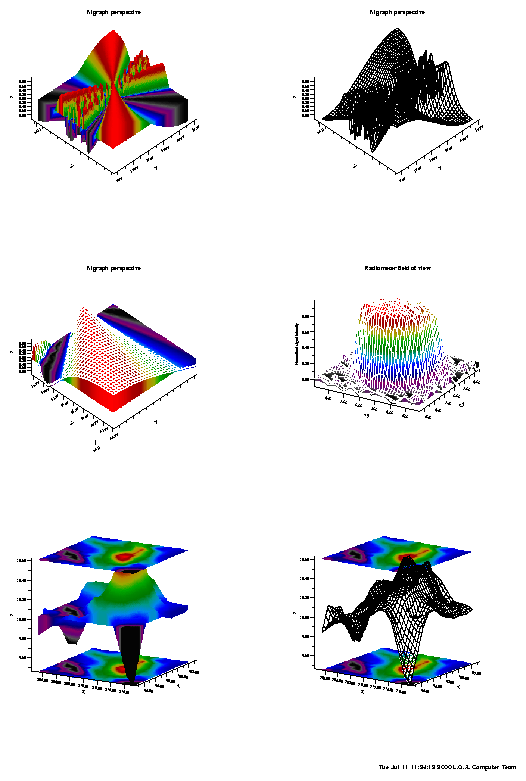
ReadSurface      File="DATA/xtract_arm19961205" Mode=IRREGULAR  \
	Ncolumns=7 Nlines=900  LinesToSkip=0 Xcolumn=3 Ycolumn=2 Zcolumn=7   UndefValue=-8421  \
	 Zmin=0 Zmax=1050

PlotTitle     Title="Rayleigh Pressure - ARM Site" Height=1.400
Grid          Frame=Yes   Xgrid=No       Ygrid=No
ContourDef  Label=No  IdealDistance=1  BackGround=transp ForeGround=Undef CFormat="%.3g" Size=1
SurfaceGeometry	 Xmin=1814 Xmax=1843 Ymin=954 Ymax=983 Interpolation=Yes DistanceFactor=1 XYRatio=1
SurfaceLUT          LutNumber=2
AddObject        Surface
ColorScale	Mode=Linear XStart=30% YStart=115% XEnd=70% YEnd=120% Min=0 Max=255 \
	 Color=Black Position=DownRight NoTick=No CFormat="%.0f" Size=1 \
	 List=0 0 500 500 1050 1050
XTitle        Title="column nbr" Height=1.400
XAxis         Scale=Linear    Min=1814    Max=1843  Delta=-1
XLabel        LabelStep=-1   Reference=-1   LabelHeight=1.600   Format=""
YTitle        Title="line nbr" Height=2.00
YAxis         Scale=Linear    Min=954    Max=983   Delta=-1
YLabel        LabelStep=-1    Reference=-1   LabelHeight=1.600   Format=""
DrawCell     XStart=1.0000   YStart=0.5000   Width=9.0000   Height=9.0000   Type=Color   Orientation=Portrait  Mode=Margin

Histogram "DATA/xtract_arm19961205" Ncolumns=7 Ycolumn=7 Nlines=900 LinesToSkip=0 Xmin=0 \
Xmax=1050 ClassSize=20 Cumulative=no YPercent=yes Style=Steps UndefValue=0

PlotTitle     Title="Rayleigh Pressure - ARM Site - histogram" Height=1.400
Grid          Frame=Yes   Xgrid=No       Ygrid=No  [Yes | Light | No]
LineStyle     Curve=1   Style=Solid           Color=Red          LineWidth=3
XTitle        Title="Rayleigh pressure (hPa)" Height=2.00
XAxis         Scale=Linear    Min=0    Max=1050  Delta=-1
XLabel        LabelStep=-1   Reference=-1   LabelHeight=1.600   Format=""
YTitle        Title=" " Height=2.00
YAxis         Scale=Linear    Min=0    Max=40    Delta=-1
YLabel        LabelStep=-1    Reference=-1   LabelHeight=1.600   Format=""
DrawCell     XStart=1.0000   YStart=10.0000   Width=9.0000   Height=9.0000   Type=Color   Orientation=Portrait  Mode=Margin


ReadSurface      File="DATA/xtract_arm19961205" Mode=IRREGULAR  \
	Ncolumns=7 Nlines=900  LinesToSkip=0 Xcolumn=3 Ycolumn=2 Zcolumn=6   UndefValue=-8421 \
	DistanceFactor=1 Zmin=0 Zmax=4

PlotTitle     Title="Phase - ARM Site" Height=1.400
Grid          Frame=Yes   Xgrid=No       Ygrid=No  [Yes | Light | No]
ContourDef  Label=No  IdealDistance=1  BackGround=transp ForeGround=Undef CFormat="%.3g" Size=1
SurfaceGeometry Xmin=1814  Xmax=1843 Ymin=954  Ymax=983 Interpolation=Yes DistanceFactor=1 XYRatio=1
SurfaceLUT          LutNumber=2
AddObject        Surface      [Region Surface Dots Triangles]
ColorScale	Mode=Boxes  XStart=30% YStart=115% XEnd=70% YEnd=120% Min=0 Max=255 \
	Color=Black Position=DownRight NoTick=No CFormat="%.0f" Size=2 \
	List=0 "clear/undet." 1  "liquid" 2  "ice" 3 "mixte"
XTitle        Title="column nbr " Height=2.00
XAxis         Scale=Linear    Min=1814    Max=1843  Delta=-1
XLabel        LabelStep=-1   Reference=-1   LabelHeight=1.60   Format=""
YTitle        Title="line nbr" Height=2.00
YAxis         Scale=Linear    Min=954    Max=983   Delta=-1
YLabel        LabelStep=-1    Reference=-1   LabelHeight=1.60   Format=""
DrawCell     XStart=11.0000   YStart=0.5000   Width=9.0000   Height=9.0000   Type=Color   Orientation=Portrait  Mode=Margin

Histogram "DATA/xtract_arm19961205" Ncolumns=7 Ycolumn=6 Nlines=900 LinesToSkip=0 Xmin=0 Xmax=4 Class=0.5 Cumulative=no  YPercent=yes Style=Steps UndefValue=0

PlotTitle     Title="Phase - ARM Site - histogram" Height=1.400
Grid          Frame=Yes   Xgrid=No       Ygrid=No  [Yes | Light | No]
LineStyle     Curve=1   Style=Solid           Color=Red          LineWidth=3
XTitle        Title=" Thermodynamic Cloud Phase  " Height=2.00
XAxis         Scale=Linear    Min=0    Max=4  Delta=-1
XLabel        LabelStep=-1   Reference=-1   LabelHeight=1.600   Format=""
YTitle        Title=" " Height=2.00
YAxis         Scale=Linear    Min=0    Max=95.8949    Delta=-1
YLabel        LabelStep=-1    Reference=-1   LabelHeight=1.600   Format=""
PlotText     XStart=61.28%  YStart=2.82%   Color=Black Style=Bold  Height=1.00 Angle=0.00  Text="0=clear/undetermined\n1=liquid\n2=ice\n3=mixed"
DrawCell     XStart=11.0000   YStart=10.0000   Width=9.0000   Height=9.0000   Type=Color   Orientation=Portrait  Mode=Margin

ReadFile     File="DATA/ARM_19961205" Mode=XY  Style=LinePlot  \
	NColumns=6  XColumn=2  YColumn=4  NLines=0  LinesToSkip=0 UndefValue=3.40282e+38

PlotTitle     Title="MMCR Data - altitude" Height=1.400
Grid          Frame=Yes   Xgrid=No       Ygrid=No  [Yes | Light | No]
LineStyle     Curve=1   Style=Solid           Color=Red          LineWidth=4
XTitle        Title="Time UTC" Height=2.00
XAxis         Scale=Linear    Min=1630    Max=1930  Delta=-1
XLabel        LabelStep=-1   Reference=-1   LabelHeight=1.60   Format=""
YTitle        Title="Cloud top Altitude" Height=2.00
YAxis         Scale=Linear    Min=0    Max=12000    Delta=-1
YLabel        LabelStep=-1    Reference=-1   LabelHeight=1.60   Format=""
DrawCell     XStart=1.0000   YStart=21.0000   Width=9.0000   Height=8.0000   Type=Color   Orientation=Portrait  Mode=Margin

ReadFile     File="DATA/ARM_19961205" Mode=XY  Style=LinePlot  \
	NColumns=6  XColumn=2  YColumn=6  NLines=0  LinesToSkip=0 UndefValue=3.40282e+38

PlotTitle     Title="MMCR Data - Temperature " Height=1.400
Grid          Frame=Yes   Xgrid=No       Ygrid=No  [Yes | Light | No]
LineStyle     Curve=1   Style=Solid           Color=Red          LineWidth=4
XTitle        Title="Time UTC" Height=2.00
XAxis         Scale=Linear    Min=1630    Max=1930  Delta=-1
XLabel        LabelStep=-1   Reference=-1   LabelHeight=1.60   Format=""
YTitle        Title="Cloud temperature (kelvin)" Height=2.00
YAxis         Scale=Linear    Min=200    Max=300    Delta=-1
YLabel        LabelStep=-1    Reference=-1   LabelHeight=1.60   Format=""
DrawCell     XStart=11.0000   YStart=21.0000   Width=9.0000   Height=8.0000   Type=Color   Orientation=Portrait  Mode=Margin

PageBox    XStart=3.7000  YStart=19.0000   Xend=12.6000   YEnd=20.6000 Color=Black Thickness=.05
PageText    XStart=4.0000  YStart=19.5000   Color=Black  Style=Plain  Height=0.4000  Angle=0.00 Text="POLDER data above the ARM site : 19961205 \nRayleigh pressure and thermodynamic cloud phase.\nARM site is located at the image center"

AddLogo    XStart=0.000 YStart=0.000 XScale=-1.000 YScale=0.000
SendToFile     File="OUT/ARM.ps"  Type=Color   Size=15.0000  Copies=1 Orientation=Portrait
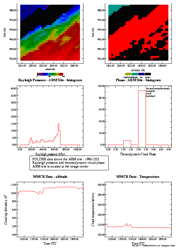
#############################################################

ReadFile      File="DATA/WORLD_MAP.gz"
ReadFile      File="DATA/Modis01.data"

PlotTitle     Title=" MODIS Land tiling for geolocated products (L2G and L3)" Height=1.00
Grid          Frame=Yes   Xgrid=Yes      Ygrid=No  [Yes | Light | No]
ScaleToFrame
LineStyle     Curve=1   Style=Solid           Color=Red          Thickness=1
LineStyle     Curve=2   Style=Solid           Color=Blue         Thickness=2

XTitle        Title=" " Height=1.50
XAxis         Scale=Formula Formula="x=x*cosd(y)"    Min=-180    Max=180  Delta=10  Label=No
YTitle        Title="Latitude" Height=1.00
YAxis         Scale=Linear    Min=-90    Max=90    Delta=10
YLabel        LabelStep=1    Reference=90   LabelHeight=0.50   CFormat="%.0f"


#   ********  Annotations ********
PlotText     XStart=0.26%  YStart=39.08%   Color=Blue Style=Bold  Height=0.40 Angle=0.00  Text="00"
PlotText     XStart=3.12%  YStart=33.54%   Color=Blue Style=Bold  Height=0.40 Angle=0.00  Text="01"
PlotText     XStart=5.98%  YStart=29.54%   Color=Blue Style=Bold  Height=0.40 Angle=0.00  Text="02"
PlotText     XStart=8.97%  YStart=26.15%   Color=Blue Style=Bold  Height=0.40 Angle=0.00  Text="03"
PlotText     XStart=11.83%  YStart=23.38%   Color=Blue Style=Bold  Height=0.40 Angle=0.00  Text="04"
PlotText     XStart=14.43%  YStart=20.92%   Color=Blue Style=Bold  Height=0.40 Angle=0.00  Text="05"
PlotText     XStart=17.17%  YStart=18.46%   Color=Blue Style=Bold  Height=0.40 Angle=0.00  Text="06"
PlotText     XStart=20.03%  YStart=16.31%   Color=Blue Style=Bold  Height=0.40 Angle=0.00  Text="07"
PlotText     XStart=22.89%  YStart=14.15%   Color=Blue Style=Bold  Height=0.40 Angle=0.00  Text="08"
PlotText     XStart=25.62%  YStart=12.31%   Color=Blue Style=Bold  Height=0.40 Angle=0.00  Text="09"
PlotText     XStart=28.35%  YStart=10.15%   Color=Blue Style=Bold  Height=0.40 Angle=0.00  Text="10"
PlotText     XStart=31.21%  YStart=8.00%   Color=Blue Style=Bold  Height=0.40 Angle=0.00  Text="11"
PlotText     XStart=33.81%  YStart=6.15%   Color=Blue Style=Bold  Height=0.40 Angle=0.00  Text="12"
PlotText     XStart=36.54%  YStart=4.31%   Color=Blue Style=Bold  Height=0.40 Angle=0.00  Text="13"
PlotText     XStart=39.40%  YStart=2.46%   Color=Blue Style=Bold  Height=0.40 Angle=0.00  Text="14"
PlotText     XStart=42.26%  YStart=0.92%   Color=Blue Style=Bold  Height=0.40 Angle=0.00  Text="15"
PlotText     XStart=44.86%  YStart=-0.62%   Color=Blue Style=Bold  Height=0.40 Angle=0.00  Text="16"
PlotText     XStart=47.85%  YStart=-2.14%   Color=Blue Style=Bold  Height=0.40 Angle=0.00  Text="17"
PlotText     XStart=50.85%  YStart=-2.14%   Color=Blue Style=Bold  Height=0.40 Angle=0.00  Text="18"
PlotText     XStart=53.71%  YStart=-0.54%   Color=Blue Style=Bold  Height=0.40 Angle=0.00  Text="19"
PlotText     XStart=56.44%  YStart=1.34%   Color=Blue Style=Bold  Height=0.40 Angle=0.00  Text="20"
PlotText     XStart=59.17%  YStart=2.95%   Color=Blue Style=Bold  Height=0.40 Angle=0.00  Text="21"
PlotText     XStart=61.77%  YStart=4.83%   Color=Blue Style=Bold  Height=0.40 Angle=0.00  Text="22"
PlotText     XStart=64.50%  YStart=6.43%   Color=Blue Style=Bold  Height=0.40 Angle=0.00  Text="23"
PlotText     XStart=67.49%  YStart=8.58%   Color=Blue Style=Bold  Height=0.40 Angle=0.00  Text="24"
PlotText     XStart=70.09%  YStart=10.19%   Color=Blue Style=Bold  Height=0.40 Angle=0.00  Text="25"
PlotText     XStart=72.95%  YStart=12.06%   Color=Blue Style=Bold  Height=0.40 Angle=0.00  Text="26"
PlotText     XStart=75.94%  YStart=14.48%   Color=Blue Style=Bold  Height=0.40 Angle=0.00  Text="27"
PlotText     XStart=78.54%  YStart=16.62%   Color=Blue Style=Bold  Height=0.40 Angle=0.00  Text="28"
PlotText     XStart=81.40%  YStart=19.03%   Color=Blue Style=Bold  Height=0.40 Angle=0.00  Text="29"
PlotText     XStart=84.27%  YStart=21.18%   Color=Blue Style=Bold  Height=0.40 Angle=0.00  Text="30"
PlotText     XStart=86.87%  YStart=23.59%   Color=Blue Style=Bold  Height=0.40 Angle=0.00  Text="31"
PlotText     XStart=89.73%  YStart=26.54%   Color=Blue Style=Bold  Height=0.40 Angle=0.00  Text="32"
PlotText     XStart=92.59%  YStart=29.76%   Color=Blue Style=Bold  Height=0.40 Angle=0.00  Text="33"
PlotText     XStart=95.19%  YStart=33.51%   Color=Blue Style=Bold  Height=0.40 Angle=0.00  Text="34"
PlotText     XStart=98.31%  YStart=39.14%   Color=Blue Style=Bold  Height=0.40 Angle=0.00  Text="35"
PlotText     XStart=49.67%  YStart=1.54%   Color=Blue Style=Bold  Height=0.40 Angle=0.00  Text="00"
PlotText     XStart=49.54%  YStart=7.08%   Color=Blue Style=Bold  Height=0.40 Angle=0.00  Text="01"
PlotText     XStart=48.11%  YStart=12.62%   Color=Blue Style=Bold  Height=0.40 Angle=0.00  Text="02"
PlotText     XStart=46.42%  YStart=17.85%   Color=Blue Style=Bold  Height=0.40 Angle=0.00  Text="03"
PlotText     XStart=44.99%  YStart=23.69%   Color=Blue Style=Bold  Height=0.40 Angle=0.00  Text="04"
PlotText     XStart=43.69%  YStart=29.23%   Color=Blue Style=Bold  Height=0.40 Angle=0.00  Text="05"
PlotText     XStart=42.52%  YStart=34.46%   Color=Blue Style=Bold  Height=0.40 Angle=0.00  Text="06"
PlotText     XStart=42.00%  YStart=40.31%   Color=Blue Style=Bold  Height=0.40 Angle=0.00  Text="07"
PlotText     XStart=42.26%  YStart=45.85%   Color=Blue Style=Bold  Height=0.40 Angle=0.00  Text="08"
PlotText     XStart=43.17%  YStart=51.38%   Color=Blue Style=Bold  Height=0.40 Angle=0.00  Text="09"
PlotText     XStart=43.95%  YStart=56.92%   Color=Blue Style=Bold  Height=0.40 Angle=0.00  Text="10"
PlotText     XStart=45.38%  YStart=62.46%   Color=Blue Style=Bold  Height=0.40 Angle=0.00  Text="11"
PlotText     XStart=46.68%  YStart=68.00%   Color=Blue Style=Bold  Height=0.40 Angle=0.00  Text="12"
PlotText     XStart=47.85%  YStart=73.54%   Color=Blue Style=Bold  Height=0.40 Angle=0.00  Text="13"
PlotText     XStart=49.02%  YStart=79.08%   Color=Blue Style=Bold  Height=0.40 Angle=0.00  Text="14"
PlotText     XStart=49.54%  YStart=84.62%   Color=Blue Style=Bold  Height=0.40 Angle=0.00  Text="15"
PlotText     XStart=49.67%  YStart=90.15%   Color=Blue Style=Bold  Height=0.40 Angle=0.00  Text="16"
PlotText     XStart=49.67%  YStart=95.08%   Color=Blue Style=Bold  Height=0.40 Angle=0.00  Text="17"
#   ********  Annotations: End ********

DrawCell   XStart=3.00   YStart=4.00   Width=15.00   Height=25.00   Type=Color   Orientation=Landscape

SendToFile     File="OUT/Modis.ps"  Type=Color
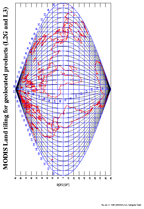
#############################################################

ReadFile      File="DATA/WORLD_MAP.gz"
ReadFile      File="DATA/Modis02A.data"

PlotTitle     Title=" MODIS coverage over USA : 7 granules - Equal-angle projection" Height=1.00
Grid          Frame=Yes   Xgrid=Yes      Ygrid=Yes  [Yes | Light | No]
ScaleToFrame
LineStyle     Curve=1   Style=Solid           Color=Red          Thickness=1
LineStyle     Curve=2   Style=Solid           Color=Blue         Thickness=4

XTitle        Title="Longitude" Height=1.00
XAxis         Scale=Linear    Min=-180    Max=-29.999  Delta=10
XLabel        LabelStep=1   Reference=-30   LabelHeight=0.70   CFormat="%.0f"
YTitle        Title="Latitude" Height=1.00
YAxis         Scale=Linear    Min=10    Max=80    Delta=5
YLabel        LabelStep=2    Reference=90   LabelHeight=0.70   CFormat="%.0f"

DrawCell        XStart=3.  YStart=3.  Width=15.  Height=12.  Type=Color

#############################################################

ReadFile      File="DATA/WORLD_MAP.gz"
ReadFile      File="DATA/Modis02B.data"

PlotTitle     Title=" MODIS coverage over USA : Tiles and granules foot prints\n(Sinusoidal projection)" Height=1.00
Grid          Frame=Yes   Xgrid=Yes      Ygrid=Yes  [Yes | Light | No]
ScaleToFrame
LineStyle     Curve=1   Style=Solid           Color=Red          Thickness=1
LineStyle     Curve=2   Style=Solid           Color=Blue         Thickness=2
LineStyle     Curve=3   Style=Solid           Color=Magenta      Thickness=4

XTitle        Title="Longitude" Height=1.00
XAxis         Scale=Formula Formula="x=x*cosd(y)" Min=-180 Max=-29.99 NewMin=-118.4 NewMax=-9.99   Delta=10
XLabel        LabelStep=1   Reference=-30   LabelHeight=0.70   CFormat="%.0f"
YTitle        Title="Latitude" Height=1.00
YAxis         Scale=Linear    Min=10    Max=80    Delta=5
YLabel        LabelStep=2    Reference=90   LabelHeight=0.70   CFormat="%.0f"


#   ********  Annotations ********
PlotText     XStart=100.48%  YStart=4.07%   Color=Blue Style=Bold  Height=0.70 Angle=0.00  Text="01"
PlotText     XStart=98.22%  YStart=19.86%   Color=Blue Style=Bold  Height=0.70 Angle=0.00  Text="02"
PlotText     XStart=94.18%  YStart=33.25%   Color=Blue Style=Bold  Height=0.70 Angle=0.00  Text="03"
PlotText     XStart=90.31%  YStart=48.56%   Color=Blue Style=Bold  Height=0.70 Angle=0.00  Text="04"
PlotText     XStart=87.08%  YStart=62.68%   Color=Blue Style=Bold  Height=0.70 Angle=0.00  Text="05"
PlotText     XStart=84.81%  YStart=77.03%   Color=Blue Style=Bold  Height=0.70 Angle=0.00  Text="06"
PlotText     XStart=83.20%  YStart=90.91%   Color=Blue Style=Bold  Height=0.70 Angle=0.00  Text="07"
PlotText     XStart=5.01%  YStart=91.15%   Color=Blue Style=Bold  Height=0.70 Angle=0.00  Text="07"
PlotText     XStart=4.85%  YStart=76.79%   Color=Blue Style=Bold  Height=0.70 Angle=0.00  Text="06"
PlotText     XStart=4.85%  YStart=62.68%   Color=Blue Style=Bold  Height=0.70 Angle=0.00  Text="05"
PlotText     XStart=4.85%  YStart=48.09%   Color=Blue Style=Bold  Height=0.70 Angle=0.00  Text="04"
PlotText     XStart=10.50%  YStart=33.01%   Color=Blue Style=Bold  Height=0.70 Angle=0.00  Text="07"
PlotText     XStart=20.03%  YStart=27.51%   Color=Blue Style=Bold  Height=0.70 Angle=0.00  Text="08"
PlotText     XStart=29.40%  YStart=22.01%   Color=Blue Style=Bold  Height=0.70 Angle=0.00  Text="09"
PlotText     XStart=38.45%  YStart=16.99%   Color=Blue Style=Bold  Height=0.70 Angle=0.00  Text="10"
PlotText     XStart=47.33%  YStart=12.44%   Color=Blue Style=Bold  Height=0.70 Angle=0.00  Text="11"
PlotText     XStart=56.87%  YStart=7.18%   Color=Blue Style=Bold  Height=0.70 Angle=0.00  Text="12"
PlotText     XStart=65.91%  YStart=2.39%   Color=Blue Style=Bold  Height=0.70 Angle=0.00  Text="13"
PlotText     XStart=75.12%  YStart=-2.39%   Color=Blue Style=Bold  Height=0.70 Angle=0.00  Text="14"
PlotText     XStart=84.98%  YStart=-4.55%   Color=Blue Style=Bold  Height=0.70 Angle=0.00  Text="15"
PlotText     XStart=94.18%  YStart=-4.55%   Color=Blue Style=Bold  Height=0.70 Angle=0.00  Text="16"
#   ********  Annotations: End ********

DrawCell        XStart=3.  YStart=16.  Width=15.  Height=11.7 Type=Color

SendToEPSFile     File="OUT/Modis.eps"  Type=Color
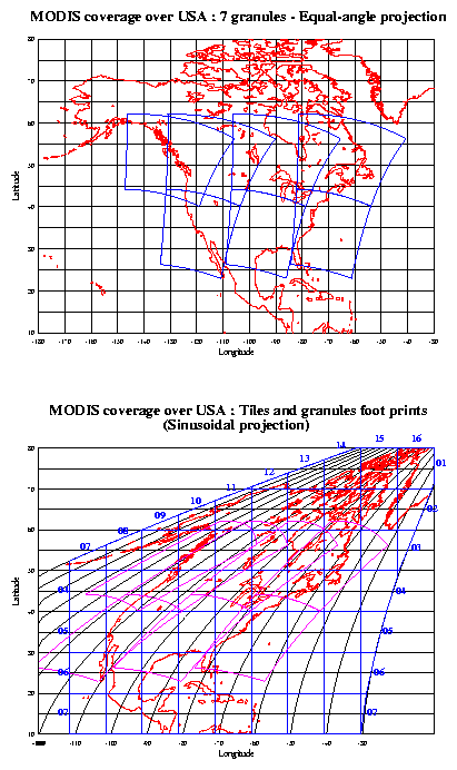
AddLogo  XStart=27. YStart=4. XScale=.1 YScale=.1

PageText 15.2 2 Black Bold 1 0 "Etude de l'angle de polarisation"
PageText 18 3.0 Black 0.5 0 "Zone : Madagascar"
PageText 18 3.6 Black 0.5 0 "Jour : 12/11/96"
PageText 18 4.2 Black 0.5 0 "Orbite : 3134"
PageText 18 4.8 Black 0.5 0 "Nombre de pixels : 26"
PageText 18 5.4 Black 0.5 0 "Coef. d'Angstr\"om moyen : 1.159"


PageText 18 6 Black 0.5 0 "$t moyen : 0.371"

# Surface
##############
ReadBinSurface File="DATA/Madagascar_12-11-96.float" DataType=Float  Ncolumns=91 Nlines=141

PlotTitle     "Situation de la sc\`ene observ\'ee" 1.10
Grid          Frame=No    Xgrid=No       Ygrid=No

SurfaceGeometry [Xmin=0 Xmax=90 Ymin=0 Ymax=140]    DistanceFactor=1 XYRatio=1 Interpolation=No
ContourDef  [Smooth=Yes|No]  BackGround=Transp [White] ForeGround=Undef [Undef|White|Black]\
	      IdealDistance=1 Size=1 CFormat="%.3g"
SurfaceLUT      File="USER_LUTS/rainbow"
SurfaceStretch          Zmin=0 Zmax=0.5 FirstLevel=0 LastLevel=255
ColorScale	Mode=Boxes [|Linear]	XStart=0% YStart=101.5% XEnd=100% YEnd=106% Min=0 Max=255 \
	Color=Black Position=DownRight NoTick=No CFormat="%.2f" Size=1.5 \
	List= 0.1 0.10 0.15 0.15 0.2 0.20 0.25 0.25 0.3 0.30 0.35 0.35 0.4 0.40 0.45 0.45 0.5 0.50
AddObject        Surface      [Region Surface Dots Triangles]
PlotBox    38 45 44 51   Black   0  5.0000
NoXLabel
XTitle        " " 1.00
XLimits        0    90
XLabel         -1    0   -1   1.00   ""
YTitle        " " 1.00
NoYLabel
YLimits        0    140
YLabel         -1    0   -1   1.00   ""
DrawCell 0.2 0.2 7.3 7 Color


#Graphe 1 a
##############

ReadFile "DATA/quv_P1L1TBG1003134BD_1" ScatterPlot 0 2 7 0 0 3.40282e+38
ReadFile "DATA/quv_P1L1TBG1003134BD_1" ScatterPlot 0 2 34 0 0 3.40282e+38
ReadFile "DATA/quv_P1L1TBG1003134BD_1" ScatterPlot 0 2 37 0 0 3.40282e+38

Grid          Frame=Yes   Xgrid=Light       Ygrid=Light  [Yes | Light | No]
PlotTitle     "Valeurs de Q \`a 865 nm\n" 1.10
LineStyle      1   NoLine   Red   1
MarkStyle      1   cross   5
LineStyle      2   NoLine   Forest   1
MarkStyle      2   cross   5
LineStyle      3   NoLine   violet   1
MarkStyle      3   cross   5
XTitle        "Angle azimutal" 1.50
XLabel         -1    -1   -1   1.00   ""
YTitle        "\nLuminance" 1.50
YLabel         -1    -1   -1   1.00   ""
#   ********  Legend drawing ********
PlotMark     2.5% -5.82%   cross   Red  5
PlotText     4% -7.35%   Black Stand  1.50 0.00"Q^{mesures}"
PlotMark     17.5% -5.82%   cross  Forest  5
PlotText     19% -7.35%   Black Stand  1.50 0.00"Q^{mod\`ele}_{sol noir}"
PlotMark     32.5% -5.82%   cross  violet  5
PlotText     34% -7.35%   Black Stand  1.50 0.00"Q^{II}_{a\'erosols}"
#   ********  Legend drawing end ********
DrawCell 0.7 7 7. 6.5 Color


# Graphe 1 b
##############

#ReadFile  FileName [Style]  Columns  XColumn  YColumn  Lines  LinesToSkip MissingValue
ReadFile "DATA/quv_P1L1TBG1003134BD_1" ScatterPlot 0 2 8 0 0 3.40282e+38
ReadFile "DATA/quv_P1L1TBG1003134BD_1" ScatterPlot 0 2 35 0 0 3.40282e+38

ReadFile "DATA/quv_P1L1TBG1003134BD_1" ScatterPlot 0 2 38 0 0 3.40282e+38
Grid          Frame=Yes   Xgrid=Light       Ygrid=Light  [Yes | Light | No]
PlotTitle     "Valeurs de U \`a 865 nm\n" 1.10
LineStyle      1   NoLine   Red   1
MarkStyle      1   cross   5
LineStyle      2   NoLine   Forest   1
MarkStyle      2   cross   5
LineStyle      3   NoLine   violet   1
MarkStyle      3   cross   5
XTitle        "Angle azimutal" 1.50
XLabel         -1    -1   -1   1.00   ""
YTitle        "\nLuminance" 1.50
YLabel         -1    -1   -1   1.00   ""
#   ********  Legend drawing ********
PlotMark     2.5% -5.82%   cross   Red  5
PlotText     4% -7.35%   Black Stand  1.50 0.00"U^{mesures}"
PlotMark     17.5% -5.82%   cross  Forest  5
PlotText     19% -7.35%   Black Stand  1.50 0.00"U^{mod\`ele}_{sol noir}"
PlotMark     32.5% -5.82%   cross  violet  5
PlotText     34% -7.35%   Black Stand  1.50 0.00"U^{II}_{a\'erosols}"
#   ********  Legend drawing end ********
DrawCell 0.7 13.6 7. 6.5 Color


# Graphe 2 a
##############

ReadFile "DATA/polar_psy_P1L1TBG1003134BD_1" ScatterPlot 0 2 9 0 0 3.40282e+38
ReadFile "DATA/polar_psy_P1L1TBG1003134BD_1" ScatterPlot 0 2 45 0 0 3.40282e+38

ReadFile "DATA/polar_psy_P1L1TBG1003134BD_1" ScatterPlot 0 2 37 0 0 3.40282e+38
Grid          Frame=Yes   Xgrid=Light       Ygrid=Light  [Yes | Light | No]
PlotTitle     "Taux de polarisation sign\'ee\n" 1.10
LineStyle      1   NoLine   Red   1
MarkStyle      1   cross   5
LineStyle      2   NoLine   Blue   1
MarkStyle      2   cross   5
LineStyle      3   NoLine   Forest   1
MarkStyle      3   cross   5
XTitle        "Angle azimutal" 1.50
XLabel         -1    -1   -1   1.00   ""
YTitle        "\nPolarisation (%)" 1.50
YLabel         -1    -1   -1   1.00   ""
#   ********  Legend drawing ********
PlotMark     2.5% -5.82%   cross   Red  5
PlotText     4% -7.35%   Black Stand  1.50 0.00"L^{mesures}"
PlotMark     17.5% -5.82%   cross  Forest  5
PlotText     19% -7.35%   Black Stand  1.50 0.00"L^{I}_{a\'erosols}"
PlotMark     32.5% -5.82%   cross  violet  5
PlotText     34% -7.35%   Black Stand  1.50 0.00"L^{II}_{a\'erosols}"
#   ********  Legend drawing end ********
DrawCell 8.0 7 7. 6.5 Color


# Graphe 2 b
##############

ReadFile "DATA/polar_psy_P1L1TBG1003134BD_1" ScatterPlot 0 2 8 0 0 3.40282e+38
ReadFile "DATA/polar_psy_P1L1TBG1003134BD_1" ScatterPlot 0 2 47 0 0 3.40282e+38

ReadFile "DATA/polar_psy_P1L1TBG1003134BD_1" ScatterPlot 0 2 39 0 0 3.40282e+38
Grid          Frame=Yes   Xgrid=No       Ygrid=Light  [Yes | Light | No]
PlotTitle     "Valeurs des angles de polarisation [0,90]\n" 1.10
LineStyle      1   NoLine   Red   1
MarkStyle      1   cross   5
LineStyle      2   NoLine   Blue   1
MarkStyle      2   cross   5
LineStyle      3   NoLine   Forest   1
MarkStyle      3   cross   5
XTitle        "Angle azimutal" 1.50
XLabel         -1    -1   -1   1.00   ""
YAxis         Scale=Formula Formula="(90*(sign(y-90)+1)-sign(y-90)*y)*2" NewMin=0 NewMax=180    Min=0    Max=180    Delta=-1
#   ********  Annotations ********
PlotAxis  Location=LEFT   Scale=Linear  Min=0  Max=90  Delta=15  \
	Color=Black  Thickness=1 Title="\nAngle de polarisation"  TitleHeight=1.50\
	LabelStep=-1 Reference=0  LabelHeight=1.00 CFormat="%2.f"
PlotAxis  Location=Right   Scale=Linear  Min=0  Max=90  Delta=15  \
	Color=Black  Thickness=1 Title=""  TitleHeight=1.50\
	LabelStep=-1 Reference=0  LabelHeight=1.00 CFormat="%2.f"
#   ********  Legend drawing ********
PlotMark     2.5% -5.82%   cross   Red  5
PlotText     4% -7.35%   Black Stand  1.50 0.00"L^{mesures}"
PlotMark     17.5% -5.82%   cross  Forest  5
PlotText     19% -7.35%   Black Stand  1.50 0.00"L^{I}_{a\'erosols}"
PlotMark     32.5% -5.82%   cross  violet  5
PlotText     34% -7.35%   Black Stand  1.50 0.00"L^{II}_{a\'erosols}"
#   ********  Legend drawing end ********
DrawCell 14.5 7 7. 6.5 Color


#Graphe 2 c
##############

Histogram "DATA/polar_psy_P1L1TBG1003134BD_1" Ncolumns=0 Ycolumn=8 Nlines=-1 LinesToSkip=0 \
	Xmin=0 Xmax=180 ClassSize=5 Cumulative=No YperCent=Yes Style=Steps UndefValue=3.40282e+38
Histogram "DATA/polar_psy_P1L1TBG1003134BD_1" Ncolumns=0 Ycolumn=47 Nlines=-1 LinesToSkip=0\
	Xmin=0 Xmax=180 ClassSize=5 Cumulative=No YperCent=Yes Style=Steps UndefValue=3.40282e+38
Histogram "DATA/polar_psy_P1L1TBG1003134BD_1" Ncolumns=0 Ycolumn=39 Nlines=-1 LinesToSkip=0 \
	Xmin=0 Xmax=180 ClassSize=5 Cumulative=No YperCent=Yes Style=Steps UndefValue=3.40282e+38
PlotTitle     Title="Histogramme des angles de polarisation\n" Height=1.10
Grid          Frame=Yes   Xgrid=Light       Ygrid=No  [Yes | Light | No]
#ScaleToFrame
LineStyle     Curve=3   Style=Solid           Color=Forest       Thickness=6
LineStyle     Curve=2   Style=Solid           Color=Blue         Thickness=4
LineStyle     Curve=1   Style=Solid           Color=Red          Thickness=2
XTitle        Title="Angle de polarisation" Height=1.50
XAxis         Scale=Linear    Min=0    Max=180  Delta=15
XLabel        LabelStep=1   Reference=-1   LabelHeight=1.00   CFormat="%.0f^o"
YTitle        Title="" Height=0
YAxis         Scale=Linear    Min=-1    Max=-1  Delta=10
YLabel        LabelStep=-1    Reference=-1   LabelHeight=1.00   CFormat="%2.f%%"
#   ********  Legend drawing ********
PlotLine     XStart=2.00% YStart=-5.10%  XEnd=5% YEnd=-5.10%  Color=Red  Style=solid  Thickness=6
PlotText     XStart=6% YStart=-7.34%   Color=Black Style=Stand  Height=1.50 Angle=0.00 Text="L^{mesures}"
PlotLine     XStart=18.00% YStart=-5.10%  XEnd=21% YEnd=-5.10%  Color=Blue  Style=solid  Thickness=3
PlotText     XStart=22% YStart=-7.34%   Color=Black Style=Stand  Height=1.50 Angle=0.00 Text="L^{I}_{a\'erosols}"
PlotLine     XStart=34.00% YStart=-5.10%  XEnd=37% YEnd=-5.10%  Color=Violet  Style=solid  Thickness=3
PlotText     XStart=38% YStart=-7.34%   Color=Black Style=Stand  Height=1.50 Angle=0.00 Text="L^{II}_{a\'erosols}"
#   ********  Legend drawing end ********
DrawCell 21.7 7 7.35 6.5 Color


# Graphe 3 a
##############

ReadFile "DATA/polar_psy_P1L1TBG1003134BD_1" ScatterPlot 0 2 37 0 0 3.40282e+38
ReadFile "DATA/polar_psy_P1L1TBG1003134BD_1" ScatterPlot 0 2 41 0 0 3.40282e+38
Grid          Frame=Yes   Xgrid=Light       Ygrid=Light  [Yes | Light | No]
PlotTitle     "Taux de polarisation sign\'ee\n" 1.10
LineStyle      1   NoLine   Forest   1
MarkStyle      1   cross   5
LineStyle      2   NoLine   Violet   1
MarkStyle      2   cross   5
XTitle        "Angle azimutal" 1.50
XLabel         -1    -1   -1   1.00   ""
YTitle        "\nPolarisation (%)" 1.50
YLabel         -1    -1   -1   1.00   ""
#   ********  Legend drawing ********
PlotMark     2.5% -5.82%   cross   Red  5
PlotText     4% -7.35%   Black Stand  1.50 0.00"L^{II}_{a\'erosols}"
PlotMark     17.5% -5.82%   cross  Forest  5
PlotText     19% -7.35%   Black Stand  1.50 0.00"L^{mod\`ele}_{sol noir}"
#   ********  Legend drawing end ********
DrawCell 8.0 13.6 7. 6.5 Color


# Graphe 3 b
##############

ReadFile "DATA/polar_psy_P1L1TBG1003134BD_1" ScatterPlot 0 2 39 0 0 3.40282e+38
ReadFile "DATA/polar_psy_P1L1TBG1003134BD_1" ScatterPlot 0 2 43 0 0 3.40282e+38

Grid          Frame=Yes   Xgrid=No       Ygrid=Light  [Yes | Light | No]
PlotTitle     "Valeurs des angles de polarisation [0,90]\n" 1.10
LineStyle      1   NoLine   Forest   1
MarkStyle      1   cross   5
LineStyle      2   NoLine   Violet   1
MarkStyle      2   cross   5
XTitle        "Angle azimutal" 1.50
XLabel         -1    -1   -1   1.00   ""
YAxis         Scale=Formula Formula="(90*(sign(y-90)+1)-sign(y-90)*y)*2" \
	NewMin=0 NewMax=180    Min=0    Max=90    Delta=-1
#   ********  Annotations ********
PlotAxis  Location=LEFT   Scale=Linear  Min=0  Max=90  Delta=15  \
	Color=Black  Thickness=1 Title="\nAngle de polarisation"  TitleHeight=1.50\
	LabelStep=-1 Reference=-1  LabelHeight=1.00 CFormat="%2.f"
PlotAxis  Location=Right   Scale=Linear  Min=0  Max=90  Delta=15  \
	Color=Black  Thickness=1 Title=""  TitleHeight=1.50\
	LabelStep=-1 Reference=0  LabelHeight=1.00 CFormat="%2.f"
#   ********  Legend drawing ********
PlotMark     2.5% -5.82%   cross   Red  5
PlotText     4% -7.35%   Black Stand  1.50 0.00"L^{II}_{a\'erosols}"
PlotMark     17.5% -5.82%   cross  Forest  5
PlotText     19% -7.35%   Black Stand  1.50 0.00"L^{mod\`ele}_{sol noir}"
#   ********  Legend drawing ********
DrawCell 14.5 13.6 7.4 6.5 Color


# Graphe 3 c
##############

Histogram "DATA/polar_psy_P1L1TBG1003134BD_1" Ncolumns=0 Ycolumn=39 Nlines=-1 LinesToSkip=0 \
	Xmin=0 Xmax=180 ClassSize=5 Cumulative=No YperCent=Yes Style=Steps UndefValue=3.40282e+38
Histogram "DATA/polar_psy_P1L1TBG1003134BD_1" Ncolumns=0 Ycolumn=43 Nlines=-1 LinesToSkip=0 \
	Xmin=0 Xmax=180 ClassSize=5 Cumulative=No YperCent=Yes Style=Steps UndefValue=3.40282e+38
PlotTitle     Title="Histogramme des angles de polarisation\n" Height=1.10
Grid          Frame=Yes   Xgrid=Light       Ygrid=No  [Yes | Light | No]
#ScaleToFrame
LineStyle     Curve=1   Style=Solid           Color=Forest          Thickness=6
LineStyle     Curve=2   Style=Solid           Color=Violet         Thickness=4
XTitle        Title="Angle de polarisation" Height=1.50
XAxis         Scale=Linear    Min=0    Max=180  Delta=15
XLabel        LabelStep=1   Reference=-1   LabelHeight=1.00   CFormat="%.0f^o"
YTitle        Title="" Height=0
YAxis         Scale=Linear    Min=-1    Max=-1  Delta=10
YLabel        LabelStep=-1    Reference=-1   LabelHeight=1.00   CFormat="%2.f%%"
#   ********  Legend drawing ********
PlotLine     XStart=2.00% YStart=-5.10%  XEnd=5% YEnd=-5.10%  Color=Forest  Style=solid  Thickness=6
PlotText     XStart=6% YStart=-7.34%   Color=Black Style=Stand  Height=1.50 Angle=0.00 Text="L^{II}_{a\'erosols}"
PlotLine     XStart=18.00% YStart=-5.10%  XEnd=21% YEnd=-5.10%  Color=Violet  Style=solid  Thickness=3
PlotText     XStart=22% YStart=-7.34%   Color=Black Style=Stand  Height=1.50 Angle=0.00 Text="L^{mod\`ele}_{sol noir}"
#   ********  Legend drawing end ********
DrawCell 21.7 13.6 7.35 6.5 Color


# Polar
##############

ReadFile "DATA/tempo_graf_position" RoTeta ScatterPlot 0  3 5 0 0 3.40282e+38
ReadFile "DATA/tempo_graf_position" RoTeta ScatterPlot 0  4 2 0 0 3.40282e+38
PlotTitle     "G\'eom\'etrie de la sc\`ene observ\'ee" 1.25
LineStyle      1   NoLine   Red   1
MarkStyle      1   Bigdot   1
LineStyle      2   NoLine   Blue   1
MarkStyle      2   Cross   1
XLimits        -90    90
XLabel         -1    -1   -1   1.00   ""
YLimits        -90    90
YLabel         -1    -1   -1   1.00   ""
Circular 0 0 90 0 0
Zenithal -8421 15 0 1 1 1 Black
Azimuthal 15 0 1 1 1 0 0 Black
#   ********  Legend drawing ********
PlotMark     -1.65% 8.57%   Bigdot   Red  1
PlotText     -0.15% 7.04%   Black Stand  1.50 0.00 " Soleil"
PlotMark     -1.65% 13.62%   Bigdot   Blue  1
PlotText     -0.15% 12.09%   Black Stand  1.50 0.00 " Satellite"
#   ********  Legend drawing end ********
DrawCell 8 0.2 6.4 7 Color


SendToFile Orientation=Landscape File="OUT/psy_P1L1TBG1003134BD_1.ps"
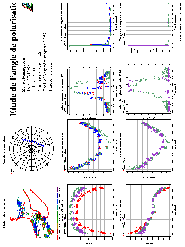
AddLogo     XStart=1.000 YStart=3.500 XScale=0.100 YScale=0.100

#############################################################

ReadFile      File="DATA/eucrex.data"

PlotTitle     Title="EUCREX MISSION 204 (April 17, 1994)" Height=0.70
Grid          Frame=Yes   Xgrid=No       Ygrid=No  [Yes | Light | No]
ScaleToFrame
LineStyle     Curve=1   Style=Solid           Color=Red          Thickness=3
LineStyle     Curve=2   Style=Solid           Color=Blue         Thickness=6
LineStyle     Curve=3   Style=Solid           Color=Blue         Thickness=6
LineStyle     Curve=4   Style=Solid           Color=Blue         Thickness=6
LineStyle     Curve=5   Style=Solid           Color=Blue         Thickness=6
LineStyle     Curve=6   Style=Solid           Color=Blue         Thickness=6
LineStyle     Curve=7   Style=Solid           Color=Black        Thickness=5
LineStyle     Curve=8   Style=Solid           Color=Black        Thickness=5
LineStyle     Curve=9   Style=Solid           Color=Black        Thickness=5

XTitle        Title="LONGITUDE" Height=1.00
XAxis         Scale=Linear    Min=-6.5    Max=-1.5  Delta=0.25
XLabel        LabelStep=4   Reference=-6.5   LabelHeight=1.00   CFormat="%1.1f^o"
YTitle        Title="LATITUDE" Height=1.00
YAxis         Scale=Linear    Min=47    Max=50    Delta=0.25
YLabel        LabelStep=4    Reference=47   LabelHeight=1.00   CFormat="%2.0f^o"


#   ********  Annotations ********
PlotText     XStart=84.43%  YStart=27.22%   Color=Black Style=Plain  Height=1.00 Angle=0.00  Text="Jersey"
PlotText     XStart=39.59%  YStart=3.55%   Color=Black Style=Plain  Height=1.00 Angle=0.00  Text="ENGLISH CHANNEL"
PlotText     XStart=63.79%  YStart=90.73%   Color=Black Style=Plain  Height=1.00 Angle=0.00  Text="Belle-Ile"
PlotBox      XStart=87.99%  YStart=87.57%  XEnd=89.12% YEnd=88.76%   Color=Black   Style=Solid  Thickness=1
PlotText     XStart=71.86%  YStart=61.14%   Color=Black Style=Plain  Height=1.20 Angle=0.00  Text="BRITTANY"
PlotText     XStart=42.03%  YStart=50.10%   Color=Black Style=Plain  Height=0.80 Angle=0.00  Text="Brest-Guipavas"
PlotText     XStart=48.78%  YStart=62.52%   Color=Black Style=Plain  Height=0.80 Angle=0.00  Text="Quimper"
PlotText     XStart=86.87%  YStart=84.22%   Color=Black Style=Plain  Height=0.80 Angle=0.00  Text="St Nazaire"
PlotText     XStart=9.01%  YStart=85.40%   Color=Black Style=Plain  Height=1.00 Angle=0.00  Text="ATLANTIC\n OCEAN\n \n"
PlotText     XStart=17.45%  YStart=50.69%   Color=Black Style=Plain  Height=1.00 Angle=0.00  Text="Ouessant"
PlotBox      XStart=48.59%  YStart=64.89%  XEnd=50.09% YEnd=66.07%   Color=Black   Style=Solid  Thickness=1
PlotBox      XStart=40.15%  YStart=52.86%  XEnd=42.03% YEnd=54.04%   Color=Black   Style=Solid  Thickness=1
PlotText     XStart=29.83%  YStart=53.65%   Color=Black Style=Plain  Height=1.00 Angle=0.00  Text="M"
PlotText     XStart=2.06%  YStart=35.31%   Color=Black Style=Plain  Height=1.00 Angle=0.00  Text="O"
#   ********  Annotations: End ********

DrawCell   XStart=2.0000   YStart=14.0000   Width=16.0000   Height=14.0000

#############################################################

#   ********  Page annotations ********
PageText    XStart=5.0000  YStart=3.5000   Color=Red  Style=Bold  Height=0.7000  \
	Text="EUCREX'94 :\n\nEuropean Cloud Radiation Experiment"
PageText    XStart=6.0000  YStart=7.0000   Color=Black  Style=Plain  Height=0.7000  \
	Text="FALCON (above the cloud) :\n\n   - Microphysical measurements\n   - POLDER downward viewing\n   - Fluxes SW and LW"
PageText    XStart=6.0000  YStart=11.5000   Color=Black  Style=Plain  Height=0.7000  \
	Text="ARAT (below the cloud):\n\n   - Lidar upward viewing\n   - Radiometer upward\n   - Fluxes SW and LW"
#   ********  Page annotations: End ********

SendToFile     File="OUT/eucrex.ps"  Type=Color
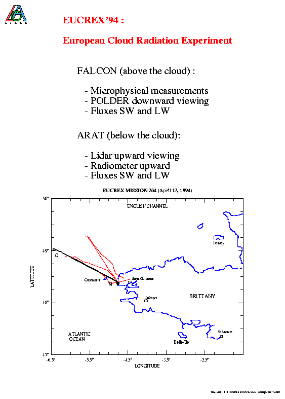
The command files hereafter were created by users of Mgraph.
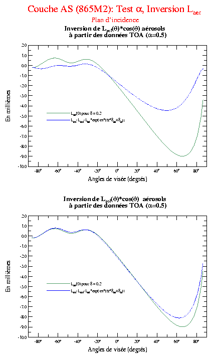
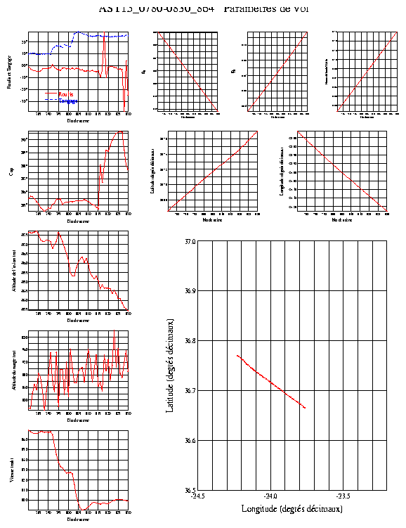
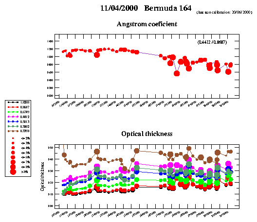
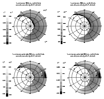
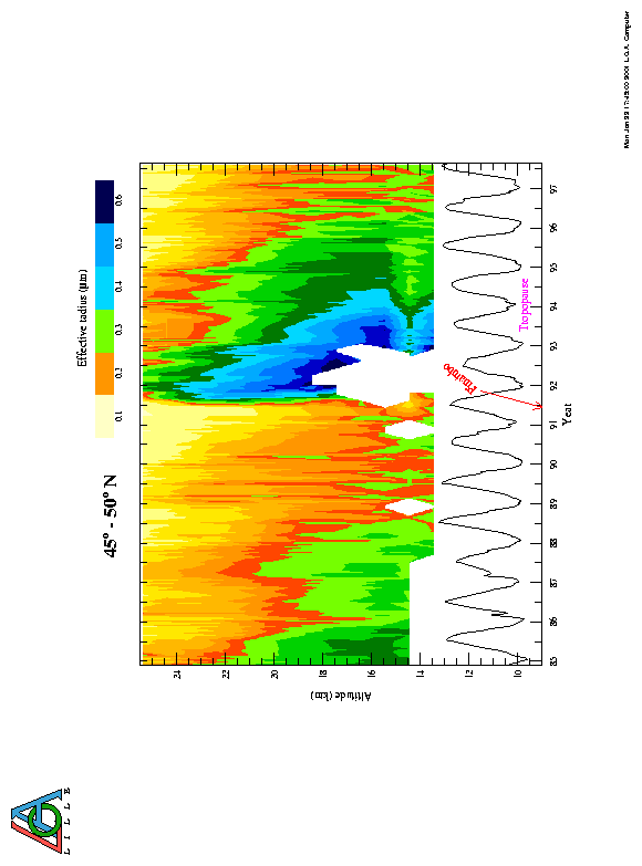
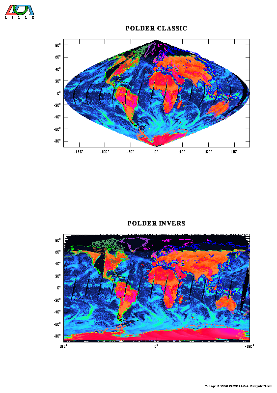
**********************************************************
AUTHORS
Gonzalez, L. Deroo, C.
Laboratoire d'Optique Atmosphérique
Université des Sciences et Technologies de Lille
U.F.R. de Physique Fondamentale
59655 Villeneuve d'Ascq Cedex
France
Email : sphinx@loa.univ-lille1.fr
The authors wish to thank: